Large language models are being asked to generate longer and longer outputs. A reasoning model may think for tens of thousands of tokens before answering a math problem ( DeepSeek-R1 ), and a coding agent may run for hours. To generate each of those tokens, the model has to look back over everything that came before, which means reading an ever-growing amount of saved state from GPU memory. For long generations, that reading dominates the cost of serving.

Sparse attention is the most direct response: at each step, read only the parts of the past that matter. It has moved from an academic idea to a production technique. DeepSeek builds it into its models ( NSA , DeepSeek-V3.2 ), and dozens of methods add it to existing models without retraining, such as Quest , H2O , and Double Sparsity .

Yet trying a new sparse attention idea in a realistic setting is painfully slow. Adding Double Sparsity to the SGLang serving engine takes roughly 2,000 lines of code, most of which reimplements basic operations like matrix multiplication and top-k selection for SGLang’s memory layout. Using a standalone research implementation instead does not help: Quest’s original code, despite its optimized kernels, runs 44.4× slower than SGLang’s ordinary full attention, so evaluating an 8B model on a single math benchmark takes nearly two hours. A sparse attention algorithm’s theoretical savings only become real speedups when it runs inside a modern serving engine, and getting it there is a substantial systems project.

This post is about Vortex, a system my collaborators and I built to remove that bottleneck. In Vortex, a sparse attention algorithm is a few lines of Python-like code, written as if there were a single request with a contiguous cache. Vortex turns it into efficient GPU code that runs inside SGLang, alongside paging, batching, and prefix caching. This makes iteration fast enough that AI coding agents can do it on their own. Given Vortex, agents wrote dozens of new sparse attention algorithms, and an 18-hour autonomous loop found a configuration that serves a reasoning workload 3.46× faster than full attention at the same accuracy.

This post is based on Vortex , to appear at NeurIPS 2026, joint work with Xinrui Zhong, Qilong Feng, Ranajoy Sadhukhan, Yang Zhou, Michael Qizhe Shieh, Zhihao Jia, and Beidi Chen. The code is open source .

Why Long Generations Are Expensive

An LLM produces text one token at a time. To generate the next token, each attention layer compares the newest token’s query vector with a key vector for every earlier token, turns those comparisons into weights, and takes a weighted average of the earlier tokens’ value vectors. Keys and values of past tokens are saved in GPU memory so they need not be recomputed. This saved state is called the KV cache .

The arithmetic per step is small: one query against \( n \) keys. But the entire KV cache must be read from GPU memory at every step, and it grows with every token generated. GPUs can do arithmetic far faster than they can read memory, so for long sequences, attention during decoding is limited by memory traffic rather than computation. Batching many requests together, the usual trick for keeping a GPU busy, does not fix this, because each request has its own KV cache to read. As one data point from our measurements: for an 8B model serving 16 requests with 32K tokens of context each, one dense attention call takes 0.76 ms, while a sparse version that reads only selected blocks takes 0.025 ms.

Sparse attention works because attention weights are usually concentrated: a query typically puts most of its weight on a small fraction of past tokens. If we can cheaply guess which ones, we can read only those and skip the rest. Static methods choose tokens by position, for example the first few tokens plus a window of recent ones ( StreamingLLM ). Dynamic methods choose based on the current query. They tend to be more accurate, but choosing then becomes part of every decoding step.

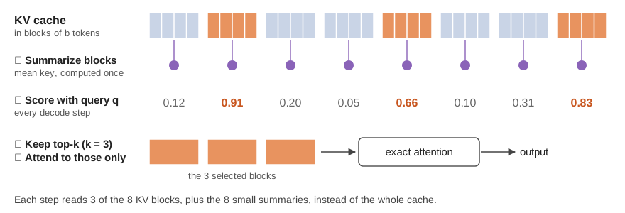
A simple dynamic method, which I will use as a running example, is block top-k attention ( Figure 1 ). Split the KV cache into blocks of \( b \) consecutive tokens and summarize each block \( j \) by its mean key \( \bar{k}_j \). At each step, score every block against the query \( q \), keep the \( k \) highest-scoring blocks \( I \), and run ordinary, exact attention over just the tokens in those blocks:

\[ s_j = q \cdot \bar{k}_j, \qquad I = \operatorname{top-}k_j (s_j), \qquad o = \operatorname{softmax}\left( \frac{q K_I^\top}{\sqrt{d}} \right) V_I . \]

Notice that there are two stages. The block summaries depend only on the keys, so they can be computed once, when a block fills up, and reused at every later step. Scoring and selection depend on the query, so they run at every step. Almost every dynamic sparse attention method has this shape, which mirrors approximate nearest-neighbor search: build a compact index ahead of time, then query it cheaply. Methods differ in what the index stores and how it is scored. Quest, for instance, stores each block’s element-wise minimum and maximum keys and uses them to bound each block’s attention score.

Why New Ideas Are Hard to Deploy

If block top-k is this simple, why does adding a new method to a serving engine take thousands of lines of code?

The answer lies in how serving engines store the KV cache. Requests have different lengths, start and finish at different times, and often share prefixes such as a common system prompt. Giving each request one contiguous buffer would waste memory, so modern engines use paged attention ( vLLM ): the KV cache lives in fixed-size pages scattered through GPU memory, and each request keeps a table listing its pages in order ( Figure 2 ). Pages can be shared between requests, which is what makes prefix caching ( SGLang ) cheap.

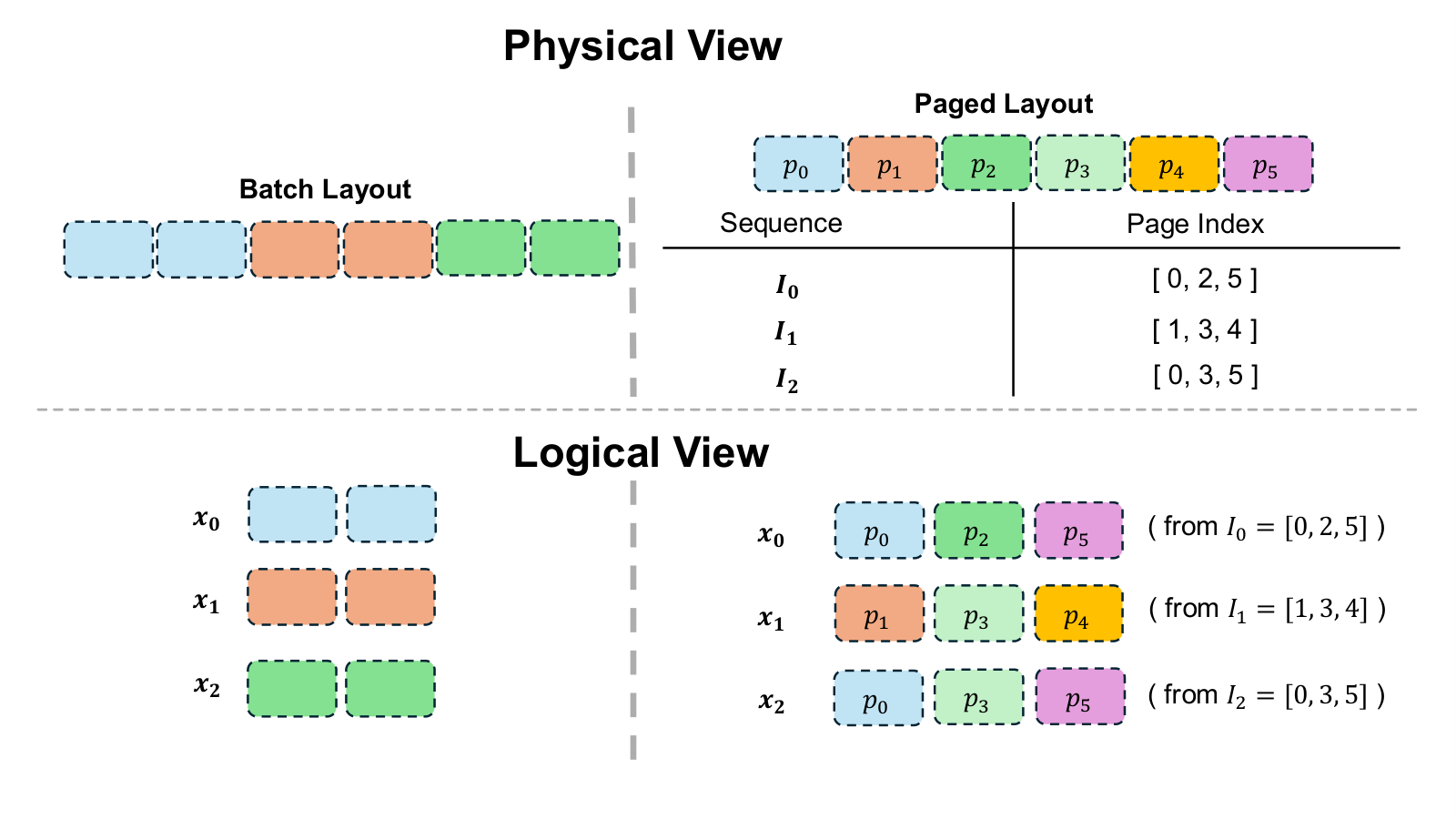
This layout breaks the assumption, built into tensor libraries like PyTorch, that a batch is a contiguous, rectangular array. An algorithm that takes a few lines of math on paper suddenly needs custom GPU code for each step: averaging keys within a page, scoring blocks spread across scattered pages, taking a top-k over a ragged set of blocks. Existing tools cover only part of this. Attention libraries such as FlashInfer and FlexAttention run attention efficiently over paged memory once you know which blocks to read. But in dynamic sparse attention, working out which blocks to read is the algorithm, and it can cost more than the attention itself. Serving engines ship a handful of built-in methods with little room for new ones. Research prototypes with hand-written kernels usually skip paging, batching, and prefix caching altogether, which is how a sparse method ends up 44× slower than the dense baseline it was meant to beat.

As a result, the people best placed to invent sparse attention algorithms, and increasingly the AI agents that could help them, spend most of their time on systems plumbing.

Vortex

Vortex splits the problem into three layers ( Figure 3 ): a small language for writing algorithms (vFlow), a tensor abstraction that understands paged memory (vTensor), and an execution backend inside SGLang.

Writing an algorithm: vFlow

In vFlow, a sparse attention method is a Python class with two functions, one for each stage described above. Here is the complete block top-k algorithm:

class BlockTopK(vFlow):
    def forward_cache(c):
        c["centroids"] = Mean(c["k"], dim=1)

    def forward_indexer(q, c):
        s = GeMM(c["centroids"], q.T)
        i = topK(Mean(s, dim=2), dim=1)
        return attn(q, c["k"], c["v"], i)

forward_cache builds the query-independent summaries and stores them in a named cache entry. forward_indexer runs at every decoding step: it scores the blocks, selects the top-k, and calls attention on the selected blocks. The key design choice is that the programmer sees a single request with contiguous tensors . Here c["k"] looks like an array of shape (1, blocks, block size, head dimension), even though in reality it is scattered across pages and shared with other requests in a batch whose makeup changes at every step. Vortex takes care of the rest.

The same small set of operators (matrix multiplication, reductions, softmax, top-k, gather, convolution, and a way to carry state from one step to the next) expresses a wide range of published methods in a few lines each. Here is the selection logic of Quest:

class Quest(vFlow):
    def forward_cache(c):
        c["max"] = Max(c["k"])
        c["min"] = Min(c["k"])

    def forward_indexer(q, c):
        s = Maximum(q * c["max"], q * c["min"])
        i = topK(Max(Sum(s)))

Double Sparsity, the block-selection branch of NSA, and H2O, which accumulates attention scores across steps, are similarly short. Static patterns are expressed by building the selected indices from positions instead of content.

Running it: vTensor

Underneath, every vFlow variable is a vTensor : an ordinary PyTorch tensor plus layout metadata, namely the batch size, an index-pointer array marking where each request’s data begins, and, for paged data, the list of pages each request uses. A vTensor operator has a simple meaning: apply the corresponding PyTorch operation to each request independently, then stitch the per-request results back into one batched tensor. For example, GeMM(c["centroids"], q.T) becomes “for each request \( i \), multiply its \( B_i \) block summaries by its query,” producing a ragged output whose length differs from request to request.

The one restriction is that operators may not mix data across requests, which matches how serving works anyway. In return, the abstraction composes: the output of any operator is a valid input to the next, with no layout conversions in between. It also has a pleasant side effect. Named cache entries like c["centroids"] are stored in pages managed by the same allocator as the KV cache, so features built on paging, such as prefix caching, keep working without any effort from the algorithm’s author.

Making it fast

A clean abstraction is only useful if it runs fast. At the start of each decoding step, the batch size and every sequence length are known, so Vortex plans the work, balancing GPU thread blocks across requests of different lengths, and generates kernels from a few templates. Operators that share a template are fused, so intermediate results such as block scores never make a round trip through GPU memory.

Top-k selection needed special care, because it is the one step that is neither a matrix multiplication nor a simple reduction. The standard radix-based top-k repeatedly buckets values by their digits, and it slows down sharply when many high scores land in the same bucket. Vortex adds two tricks. A monotonic remapping of the scores spreads them more evenly across buckets, and a stochastic early exit stops refining once it has enough confident winners, sampling the rest from the boundary bucket. At over 97% recall of the true top-k, the result is 1.30–1.62× faster than exact radix top-k (1.49× on average).

Finally, Vortex does not reimplement attention itself. It passes the selected blocks to existing, heavily optimized attention kernels from FlashInfer and TensorRT-LLM , inheriting their support for attention variants and low-precision formats. Where vendor kernels do not support a model’s shapes, as with the latent attention model discussed below, Vortex supplies its own kernel. The added overhead is small: the summary-building and selection kernels take a few microseconds, compared with hundreds of microseconds for dense attention at long contexts.

What This Makes Possible

AI agents as sparse attention researchers

If writing a new algorithm takes ten lines and testing it at serving scale takes minutes rather than days, the cycle of proposing, implementing, and evaluating ideas becomes cheap enough to hand to an AI agent. We ran two experiments, both with Qwen3-1.7B on one NVIDIA H200 GPU, measuring accuracy on competition math benchmarks (AMC23 and AIME24, generating up to 16K tokens) alongside serving throughput. The agents received Vortex’s documentation and eight representative sparse attention papers.

One-shot invention. We asked three agents, Claude Opus 4.7 and Claude Sonnet 4.6 through Claude Code and GPT-5.5 through Codex , to each propose and implement 20 new sparse attention algorithms. All 60 compiled and ran in Vortex without manual fixes. They were also genuinely different from each other: a structural distance computed from the programs’ syntax trees averaged 0.71–0.79 (out of 1) within each agent’s set. Some ideas were inventive. One scores blocks by how quickly their relevance is rising, another weights each block’s score by the magnitude of its values, and another smooths scores along the sequence so that isolated spikes are ignored. All three agents came up with that last idea independently. After staged filtering, first on a long-context retrieval benchmark ( RULER ) and then on the math benchmarks, every agent produced algorithms that match full-attention accuracy with 2–3.1× higher throughput.

Long-horizon iteration. Next, we let Claude Code with Claude Opus 4.7 run an 18-hour autonomous loop on AIME24, free to change anything: the selection rule, block sizes, the KV cache’s numeric format, or which layers stay dense. Over 23 iterations and 92 submissions ( Figure 4 ), it found a configuration that serves 11,894 tokens per second versus 3,437 for full attention, a 3.46× speedup, at the same accuracy (38.96% versus 38.54%).

It is worth being clear about what the agent did and did not do. Its best final algorithms converged back to block top-k, improved through tuned block sizes, selection strategies, and skipped layers, rather than a fundamentally new mechanism. Along the way it tested many diverse ideas, many of which beat full attention. Inventing a fundamentally better sparse attention algorithm remains an open problem. What Vortex changes is that an agent can now run dozens of realistic, end-to-end experiments on its own, which is a prerequisite for getting there.

Designing for a new architecture

Some of the newest models do not use standard attention at all. DeepSeek and GLM models use multi-head latent attention (MLA) ( DeepSeek-V2 ), which compresses each token’s keys and values into a small latent vector plus a separate component that carries positional information (the rotary embedding, or “rope”). Existing sparse attention methods were designed for standard attention, and MLA’s compressed layout is exactly the kind of detail that makes prototyping painful.

With Vortex, we designed a rope-aware block-sparse method for MLA that scores each block using both the compressed content and the positional component. On GLM-4.7-Flash ( GLM ), generating up to 32K tokens for AIME26 problems on one NVIDIA B200 GPU, full attention reaches a mean accuracy of 0.765 at 1,031 tokens per second. The rope-aware method comes within about a point (0.752) at roughly 4× the throughput, reaches up to 4.7× with a tighter block budget, and matches or beats full attention on pass@4 and pass@8 ( Figure 5 ). Quest stays behind it throughout. One caveat: the vendor’s optimized MLA kernel does not support this model’s head shapes, so the full-attention baseline falls back to a slower kernel, while the sparse methods run on Vortex’s own MLA kernel. Part of the gap therefore reflects kernel support, not sparsity alone.

The ablation in the same figure is revealing. A rope-unaware variant, which scores blocks from the compressed content alone, drops to 0.60–0.63 accuracy. The positional component, not just the content, carries the signal needed to pick the right blocks.

Learning where the signal lives

That result points to a third use: Vortex as a research instrument. Because a scoring rule is a few lines of code, we can run controlled experiments on which parts of the key representation actually drive block selection.

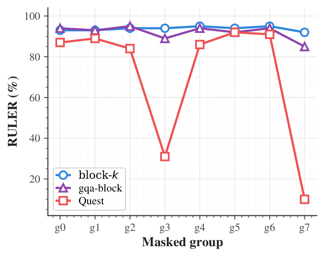
In Qwen3-4B and Qwen3-8B ( Qwen3 ), we split the 128 query-key channels into eight groups of 16 and masked one group at a time during block selection, measuring accuracy on RULER ( Figure 6 ). The routing signal turned out to be highly concentrated: only two groups, g3 and g7, matter. Masking either one alone barely affects block top-k, although Quest collapses. Masking both collapses every method to near-random, even with six of the eight groups intact. Conversely, keeping only the half of the channels that contains g3 and g7 loses nothing. The same two groups matter at both model sizes, which suggests a property of the Qwen3 family rather than a quirk of one model, though we have not checked whether it carries over to other families.

Is it actually fast?

Everything above depends on Vortex delivering real end-to-end speedups, so we measured them directly against full attention in SGLang, the engine Vortex is built into. On Qwen3 models from 0.6B to 8B parameters on an H200, with inputs up to 4K tokens and outputs up to 16K, we swept the number of blocks each query attends to (the top-k budget) from 256 down to 32 and traced the throughput–accuracy frontier ( Figure 7a ). Allowing up to 5 points of accuracy loss, block top-k reaches 3.46× (AMC23) and 3.60× (AIME24) the throughput of full attention, and Quest reaches 2.73× and 2.98×. Under a stricter 1-point budget, block top-k still delivers 2.14–2.31× on AMC23 and 2.42–3.60× on AIME24, depending on model size.

Faster decoding also means lower latency for users under load. With 16K-token prompts arriving at up to 8 requests per second, in a setup that runs prefill and decoding on separate GPUs to isolate decoding, sparse attention cuts the 95th-percentile time per output token by up to 11.7× with block top-k and 12.8× with Quest ( Figure 7b ).

The gains persist at large scale, though they shrink. On MiniMax-M2.7 ( MiniMax-M2 ), a 229-billion-parameter mixture-of-experts model served across four B200 GPUs, full attention reaches 0.83 accuracy at 3,341 tokens per second on AIME26 with 32K-token generations. Block top-k slightly exceeds that accuracy (0.84) at 1.23× the throughput, and reaches 1.37× with a tighter budget. The gains are smaller because, at this scale, more of each decoding step goes to reading model weights and communicating between GPUs rather than to reading the KV cache.

Across all of these sweeps, one practical default emerged: blocks of 16 tokens with about 125 selected blocks sit near the accuracy ceiling while keeping most of the speedup.

Limitations

Vortex currently accelerates only decoding, not the prefill phase that processes the prompt, and only inference, not training, where sparse attention would also need a backward pass. It targets attention models with an explicit KV cache; extending the abstraction to recurrent and state-space models such as Mamba is future work. And although Vortex makes experiments cheap, it is not itself an autonomous research system: our longest agent run refined a known algorithm rather than inventing a new one.

Conclusion

Progress in sparse attention has been limited less by ideas than by the engineering needed to test them where they matter, inside a real serving engine. Vortex lowers that cost: algorithms are written against a simple single-request view, and a paged tensor abstraction and an optimized backend handle everything else. The result makes human researchers faster, lets AI agents explore the design space on their own, and doubles as an instrument for understanding why sparse attention works. As generations grow longer and agents take on more of the research loop, I expect the ability to turn a ten-line idea into a realistic measurement within minutes to matter more and more.