Modern machine learning (ML) kernels evolve rapidly with new optimizations and hardware features. ML compilers must accommodate richer memory hierarchies, more forms of thread cooperation, and backends with different execution models, while retaining the control needed for peak performance.

We built TIRx , an ML compiler for GPUs and AI accelerators based on Apache TVM, around three explicit interfaces. Execution scope describes the hardware teams participating in an operation, from individual threads to clusters of thread blocks. Tensor layouts map tensor indices to physical locations through named hardware axes, with explicit sharding, replication, and offsets. Tile primitive dispatch then uses the scope, layouts, and backend to turn operations such as copying data and multiplying matrices into efficient instruction sequences.

This design preserves native-level control while automating recurring address calculations, operand preparation, and instruction-loop generation. Programmers still choose the memory allocation, thread assignments, pipeline, and synchronization, and can use hardware instructions directly. Our evaluation on NVIDIA B200 and AWS Trainium1 shows performance competitive with that of vendor and hand-tuned libraries. Comparisons with native implementations also show substantial reductions in low-level code.

Why we built TIRx

In Python, multiplying two matrices takes one expression: C = A @ B . On the latest hardware, such as NVIDIA Blackwell GPUs, the program that implements it, called a kernel , can contain thousands of lines of code. Much of that code moves data between memory spaces, divides work among threads, and coordinates their execution.

Each output element in C = A × B is a dot product: multiply a row of A by a column of B , then sum the products. Computing each output independently would load the same inputs many times. Kernels therefore work on tiles , small rectangular regions whose values can be reused in fast memory.

On NVIDIA GPUs, global memory holds the full matrices, shared memory holds tiles accessible to a block of threads, and each thread has private registers. Blackwell adds tensor memory , a separate on-chip memory with two-dimensional addressing. A value in global or shared memory is located by its memory offset. Locating a value in registers requires a thread ID and a register slot. Blackwell tensor memory instead uses two coordinates, Lane and Col . Some instructions also require copies of the same value in several locations.

The threads moving and processing these tiles can have different jobs. NVIDIA groups threads into warps of 32, with several warps in a thread block. Some warps can fetch tile k+1 while others compute on tile k , an arrangement called warp specialization . Hardware also supports cooperation among pairs and clusters of thread blocks. In some cases, one thread issues an instruction on behalf of a much larger team. The compiler must distinguish that team from the threads that actually execute the call.

Moving to another accelerator changes how code executes and how data is stored. AWS Trainium, for example, exposes a single-thread programming model with explicitly managed on-chip buffers. The buffers have their own dimensional constraints, and work is no longer distributed over GPU warps.

Programmers can use these hardware features by calling native instructions directly. But they must also calculate addresses, prepare operands, and write loops to apply those instructions across a tile. Repeating this work across kernels creates boilerplate that is difficult to maintain and easy to get wrong. A compiler can automate this work through reusable tile operations. To do so, it needs to know the operands’ storage layouts and the participating hardware team, then check both against the target instruction’s requirements. It can then generate the implementation of each tile operation while leaving the surrounding pipeline and synchronization under the programmer’s control.

The table compares four approaches to kernel programming. Multi-vendor support describes which backends a system provides; kernel portability describes how much the source must change when moving between them. Programming granularity refers to the basic execution level exposed by the language, even when its collective operations involve larger teams.

	Triton	Gluon	CuTe DSL	TIRx
Abstraction	Abstract tiles	Tiles with layouts	PTX-level operations + layout utilities	Native code (CUDA/NKI) + tiles with layouts
Programming granularity	Block	Warp partitions	Thread	Thread
Performance potential*	≈80% SOL or higher	Near SOL	Near SOL	Near SOL
Multi-vendor support	Yes	Yes	No	Yes
Kernel portability	Usually	Manual porting	Manual porting	Manual porting
Layouts	Hidden	Linear layouts	CuTe layouts	Axe layouts (named axes)

SOL (“speed of light”) denotes the hardware performance limit for a workload. The performance row is our rough expectation for tuned kernels; actual results depend on the operation, shape, and device. The evaluation reports our measurements.

PTX is NVIDIA’s virtual instruction set for GPUs. NKI (Neuron Kernel Interface) is AWS’s low-level interface for writing Trainium kernels. Axe layouts are TIRx’s layouts with named hardware axes; the layout section explains their notation.

Existing systems divide this work differently. Triton lets programmers write block operations and leaves much of the per-thread implementation to the compiler. Gluon provides more explicit control over layouts and hardware operations. CuTe DSL exposes atoms that mirror hardware instructions; programmers use layout operations to partition tensors into the portions handled by each thread. We built TIRx to combine native-level kernel programming with reusable tile operations. Each tile operation acts collectively over the team specified by its execution scope. Programmers choose the operand layouts and the surrounding kernel schedule; dispatch derives each thread’s work from those layouts.

We start with two sums that differ in how threads cooperate, then use layout notation to describe memory addresses and thread ownership. With both descriptions in place, we can see how dispatch selects and implements each tile operation.

Execution scope: who participates?

Suppose all 32 threads in a warp are active. They hold the integers 1 through 64 in registers, two consecutive values per thread. We can compute two different kinds of sums from these same values.

One sum per thread. Each thread adds its own two values: thread 0 computes 1 + 2 = 3 , thread 1 computes 3 + 4 = 7 , and so on. There are 32 independent reductions and 32 results. Each thread can compute its result using only its own registers.

One sum for the warp. The threads collectively sum all 64 values, producing one logical result, 2080 . This reduction must combine values held by different threads. All 32 threads participate in one operation.

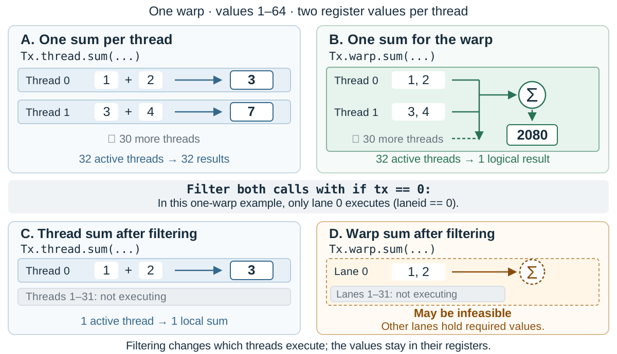
Figure 1. Team kind and filtering are separate choices. Top: all 32 threads execute. Bottom: if tx == 0 selects only lane 0 in this single-warp example. Its thread sum can run; the warp sum may be infeasible because it still needs the other lanes’ values.

The two operations in the top row run on the same threads, but they group the work differently. TIRx records both facts in its execution scope . The active thread set identifies the threads executing the call: all 32 threads in both top panels. The team kind specifies the granularity of the operation: thread in the first example, warp in the second. Other team kinds include warpgroup (four consecutive warps on NVIDIA GPUs), block, and cluster.

Each call specifies its team kind through its prefix: Tx.thread.sum(...) computes the independent per-thread sums, while Tx.warp.sum(...) computes the collective warp sum. Ordinary control flow determines which threads reach the call. In this single-warp example, tx ranges from 0 to 31, so if tx == 0: leaves only lane 0 active, just as if laneid == 0: would.

The bottom row shows what happens under this condition. A Tx.thread.sum(...) call can still add lane 0’s own values to get 3. The warp sum shown here still needs values held by the other lanes, so placing Tx.warp.sum(...) under the same condition may be infeasible. Filtering changes the active thread set while keeping the team kind unchanged. Dispatch checks that the active threads and operand layouts satisfy the operation’s hardware requirements.

Tensor layouts: where values live

Execution scope specifies the threads and team for an operation. The compiler also needs to know where each operand’s values are stored. A tensor layout maps a logical index to its storage locations.

Conventional layouts

For a row-major 8 × 16 array, we write the layout as:

(8, 16):(16, 1)

The tuple before the colon gives the dimension sizes: 8 rows and 16 columns. The tuple after it gives the strides. Increasing the row index by one advances the memory offset by 16 elements; increasing the column index by one advances it by one element. Element (i, j) therefore has offset 16*i + j , and (3, 9) has offset 57.

TIRx extends this notation by attaching a hardware axis to each stride. With m denoting a linear memory coordinate, the same layout is (8, 16):(16@m, 1@m) . An omitted axis defaults to m .

Multidimensional buffers: TMEM

Some on-chip memories use several physical coordinates to address a value. Blackwell tensor memory , or TMEM, uses Lane and Col . Here Lane is a memory coordinate, separate from a thread’s lane ID. We can describe this two-dimensional storage by assigning strides to these two axes. For example, the following layout spans 128 lanes and 224 columns:

(2, 128, 112):(112@Col, 1@Lane, 1@Col)

The middle index selects one of 128 Lane coordinates. The last index selects one of 112 columns. The first index adds either 0 or 112 to the column coordinate, placing two groups of 112 columns next to each other. For a logical index (a, i, j) , the physical coordinates are:

Lane = i
Col  = 112*a + j

Thread ownership

The same notation can describe which thread owns a value. For register storage, we need a warp ID, a lane ID (the thread’s position within its warp), and a register slot. The example below distributes an 8 × 16 tile over two warps and replicates it in two more. In each copy, one warp holds the left eight columns and another holds the right eight. Each warp stores 64 values across 32 lanes, giving two values per lane.

Figure 2 shows the arrangement. Warps 5–6 hold one copy, and warps 9–10 hold the other. Within each half-row, four lanes each hold two adjacent values. The layout specifies both the spacing between copies and their starting position in the block.

Figure 2. Register layout from our paper. L0 – L31 label lanes, and R0 and R1 label register slots. Blue cells belong to warps 5 and 9; peach cells belong to warps 6 and 10. Warps 5–6 and warps 9–10 each hold a complete copy of the 8 × 16 tile.

Using the hardware-axis names in Figure 2, we can write the complete layout as:

D[(8, 2, 4, 2):(4@lane, 1@warp, 1@lane, 1@reg)]
+ R[2:4@warp]
+ 5@warp

Shard ( D ). The row dimension contributes the first extent, 8. The 16-column dimension is factored into 2 × 4 × 2 , giving the remaining extents. Each extent is paired with the stride in the same position. The rows use 4@lane , so advancing one row advances four lanes. The column factors use 1@warp , 1@lane , and 1@reg : they select one of two warps, one of four lanes within a half-row, and one of two register slots. This places one copy of the tile in warps 0 and 1 before replication and offset are added.

Replica ( R ). R[2:4@warp] specifies two copies separated by four warps. It adds warp displacements of 0 and 4, placing the copies in warps 0–1 and 4–5.

Offset ( O ). 5@warp shifts all these coordinates by five warps. The copies therefore occupy warps 5–6 and 9–10, as in the figure.

Expanding this layout gives the register coordinates of element (i, j) :

lane          = 4*i + (j // 2) % 4
register slot = j % 2
warp          = 5 + j // 8, or 9 + j // 8

For (3, 9) , the shard gives lane 4*3 + (9 // 2) % 4 = 12 , register slot 9 % 2 = 1 , and warp 9 // 8 = 1 . Adding the replica displacements and the fixed offset gives warps 1 + 0 + 5 = 6 and 1 + 4 + 5 = 10 . The same logical value thus occupies register slot 1 of lane 12 in both warps.

In general, the three components define the mapping:

$$ L(x) = {D(x) + r + O \mid r \in R}. $$

Here x is a logical index. The result is a set because an element can have more than one storage location. Common layouts are available through library helpers, and programmers can define their own when needed.

Why this layout design

General shapes. Non-power-of-two dimensions are common in global-memory tensors and in buffers within a kernel, including shared-memory buffers that hold several pipeline stages. On-chip capacity can also make a non-power-of-two tile useful, as with the 224-column TMEM tile above. TIRx’s shape-and-stride representation supports these sizes directly.

Logical to physical mapping. We could instead map physical locations to logical indices. Replication would then be straightforward: several locations would each map to the same logical element. But a strided tensor can leave gaps in physical storage. Those unused locations have no element of that tensor to map to. TIRx starts from a logical element and describes the locations that hold it, using the replica component when there is more than one.

Explicit hardware axes. A generic thread coordinate leaves another question open: which group of threads does it refer to? Consider this layout, where t stands for a thread coordinate and m for a memory coordinate:

(128, 4):(1@t, 1@m)

Here t could mean a thread ID within the whole block, or an ID local to a warpgroup. The same expression would then describe different placements. To distinguish them, the compiler would need extra information attached to the tensor, or a convention such as inheriting the meaning of t from the execution scope where the tensor was defined.

TIRx names the coordinate explicitly. The two cases become:

(128, 4):(1@tid,       1@m)
(128, 4):(1@tid_in_wg, 1@m)

The first uses thread IDs within a block; the second uses thread IDs within a warpgroup. The choice is part of the layout itself.

Tile primitive dispatch: from operations to instructions

At compile time, tile primitive dispatch chooses a family of hardware instructions using the operation, target hardware, operand storage spaces, execution scope, and explicit configuration. The selected family’s rule checks whether the layouts, shapes, types, and alignment meet its requirements. Compilation fails if no legal implementation is available.

Consider the two sums in Figure 1. The layout tells dispatch that each thread holds two values in registers. The thread-scoped call needs only a local addition. For the warp-scoped call, TIRx supports a warp-shuffle implementation: threads can read register values from other lanes in the warp. The implementation can first add each thread’s two values, then exchange and add these partial sums across lanes. The team kind determines whether the reduction combines values across threads; the layout identifies the registers holding those values.

Preparing operands can require slicing a tile, regrouping its dimensions, or permuting its logical axes to produce the view an instruction expects. Within the selected family, dispatch chooses the largest legal instruction shape unless the programmer requests another legal shape. It generates addresses and loops to cover the parts of the tile that one instruction cannot handle at once.

TIRx’s programming model: native code with tile dispatch

Programmers write the kernel’s control flow, allocate buffers, assign work to threads, and arrange the pipeline. They can mix direct hardware instruction calls with tile operations in the same kernel.

Figure 3 shows the producer that loads input tiles for a matrix multiplication. The if statements assign this role to a warp, and elect_sync() selects an issuing thread. The loop, barrier wait, and pipeline-state updates remain explicit. The three Tx.copy_async calls transfer tiles from global-memory tensors A and B to shared-memory buffers Asmem and Bsmem . Their configuration selects NVIDIA’s Tensor Memory Accelerator (TMA), which performs the transfers asynchronously.

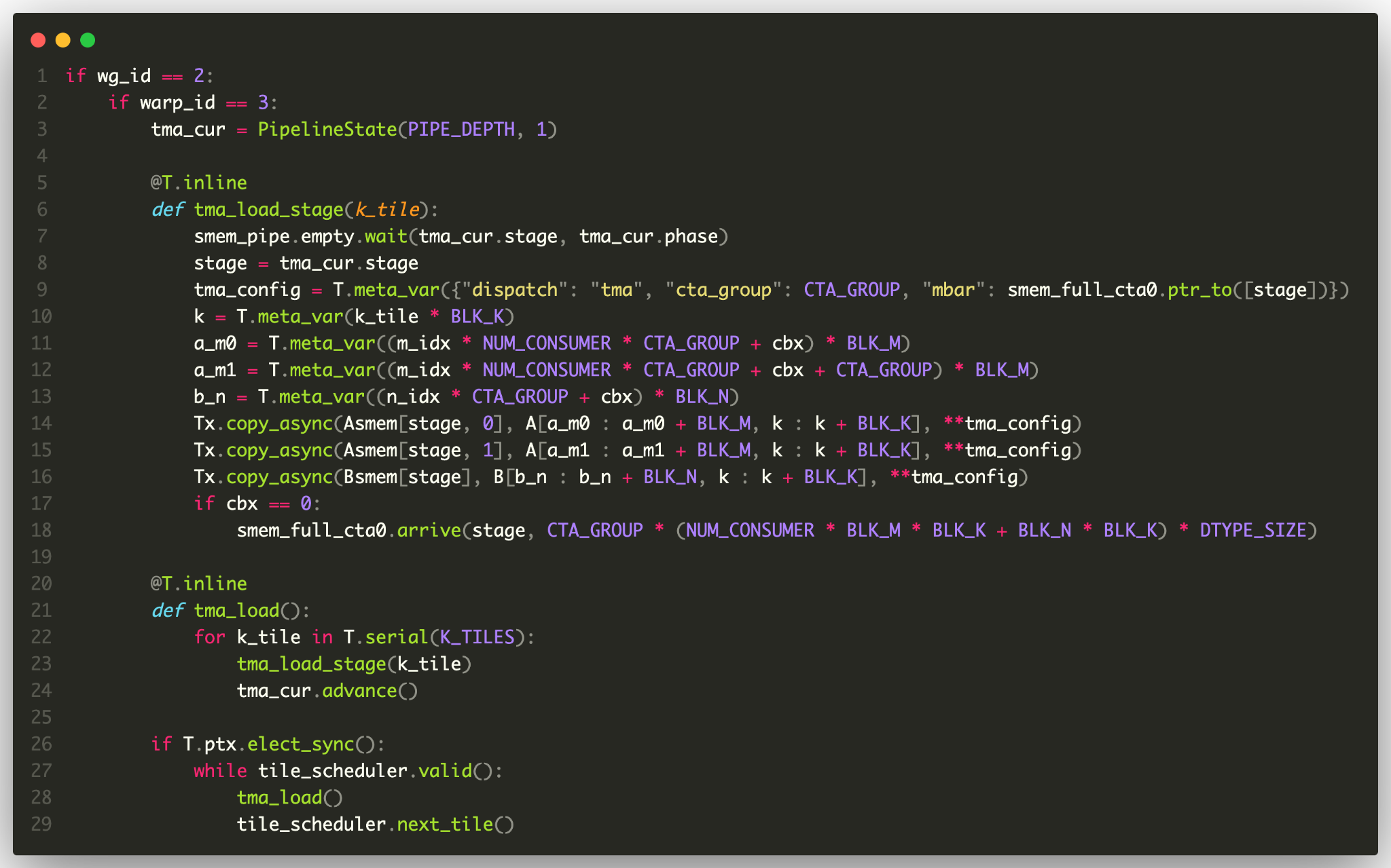
Figure 3. Producer code from the June launch article . Control flow and pipeline synchronization are explicit; tile copies use dispatch. The original excerpt uses that article’s unqualified Tx.copy_async for thread-scoped calls.

Each tile operation is dispatched independently using its scope, operand layouts, and configuration. Programmers choose the logical tile and can request a particular instruction family or legal instruction shape. Dispatch prepares the operands and generates instruction loops for that call; the surrounding code determines when it runs and how it is synchronized.

For asynchronous operations, the programmer explicitly selects the instruction family and writes the corresponding waits before consuming results or reusing buffers. Dispatch must honor that choice, because different instruction families can require different synchronization protocols.

Evaluation

We evaluated matrix multiplication and attention kernels on NVIDIA B200 and AWS Trainium1 to compare their performance with that of vendor and hand-tuned libraries. We then compared implementations to see how much low-level code the tile primitives replace and which scheduling code remains explicit.

Kernel performance

The table shows selected B200 results from our paper . FP16 and FP8 denote 16-bit and 8-bit floating-point values. In FP8 block-scaled matrix multiplication, groups of input values share scale factors that adjust their numerical range. Attention combines values across positions in a sequence; causal attention excludes future positions. Throughput is reported relative to the baseline, with 1.00× meaning equal throughput.

Workload	Baseline	TIRx result
FP16 matrix multiplication	cuBLAS	Within 4% on average
FP8 block-scaled matrix multiplication	DeepGEMM	About 0.92–1.00× across eight shapes
Non-causal attention, head dimension 128	FlashAttention-4	1.00× on average
Causal attention, head dimension 128	FlashAttention-4	About 0.96× on average

We used CUDA 13.0 and driver 580.82.07. The matrix multiplications use M = 8192 and model-derived weight shapes. The FP8 baseline is DeepGEMM commit 11cbe26 ; the range above is computed from the eight pairs of throughput values in the paper’s GEMM figure. The attention tests use 128 values per head vector and sequence lengths from 1K to 32K.

On Trainium1, our kernels match the performance of the handcrafted Neuron Kernel Interface (NKI) library on the square matrix multiplications we tested. For non-causal attention, we obtain a 1.26× average speedup over NKI. The speedup comes from our choice of pipeline schedule and memory allocation.

Case study

The FP8 kernel above uses about 250 lines of Python, compared with roughly 550 lines of CUDA C++ in DeepGEMM. TIRx generates much of the code for address calculations, along with loops that apply an instruction repeatedly across a tile.

Our FlashAttention-4 implementation provides a more specific example. It has only one user-declared layout, which describes register placement for tensor-memory transfers. For a conditional tensor-memory-to-register load, the CuTe DSL implementation explicitly composes and slices layouts to obtain each thread’s portion of the source and destination tensors, then issues the copy. TIRx expresses the same transfer as one collective copy over the participating thread team. Dispatch derives the per-thread implementation from the execution scope and operand layouts. The warp-specialized schedule, asynchronous pipeline, and per-thread exponential approximation remain explicit in TIRx.

The comparison with Triton shows what explicit scheduling offers in return for more code. Our FP16 kernel uses about 180 lines of Python, compared with about 80 in Triton. We explicitly assign work to warps and coordinate pairs of thread blocks, whereas the evaluated Triton kernel leaves scheduling to the compiler and uses no cluster cooperation. On B200, our kernel comes within about 4% of cuBLAS throughput on average; Triton trails cuBLAS by roughly 9–12% on most tested shapes.

Limitations

Runtime-dependent team membership or ownership. Collective dispatch needs a statically representable team and a mapping that describes which threads own each value. Dynamic spatial partitioning or work stealing may instead determine team membership or tile ownership at runtime. That scheduling decision falls outside the collective dispatch contract.

Position-dependent strides. A stride can be determined at runtime, as long as its value is uniform along the corresponding logical dimension. A layout with a different row stride for each row falls outside this representation.

Programmers can implement dynamic scheduling and irregular address calculations directly in native code while using tile primitives for compatible operations in the same kernel. Dispatch uses their scopes and layouts to generate addresses, prepare operands, and build instruction loops; programmers retain control of the kernel’s schedule and synchronization.

Acknowledgments and further reading

This post is based on our paper, Bohan Hou et al., TIRx: A Unified Tile Primitive ML Compiler Across Heterogeneous Backends , ASPLOS 2027 .

The work was done with Hongyi Jin, Guanjie Wang, Shushi Hong, Jinqi Chen, Yaxing Cai, Lijie Yang, Zihao Ye, Yaoyao Ding, Ruihang Lai, Todd C. Mowry, and Tianqi Chen. TIRx builds on Apache TVM and the community’s work on kernel languages and tensor layouts.

The TIRx documentation and community kernel examples are good starting points for trying it. The compiler is in the Apache TVM repository ; the June 2026 launch article covers more of the project’s design and applications.