
The Online Reviewer Assignment Problem
Paper submission volumes have been increasing in recent years. Submissions to the largest ML conferences have grown 2-4x in just the last 3 years! Conferences and journals have to maintain the scale of peer review, even as it may become infeasible for program chairs and editors to assess reviewers’ expertise. Many conferences have adopted automated paper-reviewer assignment systems to cope with increasing submission volumes. In contrast, most journals continue to match papers to reviewers manually. This post is about automating journal paper-reviewer assignment.
How do we currently automate paper-reviewer matching?
Automated paper-reviewer assignment algorithms have to get two things right.
- Quantifying the match quality of any (paper, reviewer) pair — how competent is the reviewer to review the given paper?
- Once we have quantified match qualities, assigning papers in a globally satisfactory way.
The first part is handled by computing a similarity score for every paper-reviewer pair: a scalar measuring the textual similarity between a submitted paper and each reviewer’s recent work. This works the same for both conferences and journals, and we have well-established ways of doing it (e.g. the Toronto Paper Matching System ).
The second part works differently for conferences and journals. In conferences, we have a batch problem: a massive set of papers must be assigned to a massive pool of reviewers in one shot. This is handled by solving a large linear program (LP). In journals, we instead have a stream of submissions which we must assign online , as they arrive, to reviewers from a pool. We don’t know when papers will arrive or what topics they’ll cover. We can’t assign the same reviewers to too many papers, to be respectful of their time. Journals that automate assignment currently assign whichever available reviewers have the best similarity score — pretty much skipping part two.
The problem with the current approach
We call this approach “Greedy”: when a paper arrives, assign the best available reviewers. While reasonable, it has a failure mode. Consider the following example.
A journal has three reviewers:
- Fei-fei ExpertLi : a veteran expert reviewer, spanning much of modern ML. Most papers rate her highly.
- Adam Stepinski : has spent his career on optimization: convergence proofs, gradient methods, the mathematics of training.
- Bayesian Beginner : a junior reviewer still developing expertise. Competent but not strong on any topic.
The journal receives two types of papers: LLM papers (80% of submissions) and optimization papers (20%). The similarity scores are:
ExpertLi is the best reviewer for both paper types. Reviews take 1 timestep after submissions. Each assigned reviewer is unavailable for the next arriving paper.
What Greedy does. An optimization paper arrives. All three are free. Greedy assigns ExpertLi. She’s now unavailable. The next paper is on LLMs, as 80% of papers are. Only Stepinski and Beginner are free. Greedy picks Stepinski over Beginner. The paper after that is also LLM, but ExpertLi is now available again. Greedy picks ExpertLi. A third LLM paper arrives, Greedy assigns to Stepinski since he is marginally more competent to review it than Beginner. Last, another Optimization paper arrives. Greedy assigns to ExpertLi.
Greedy tries to assign ExpertLi whenever she is available, underutilizing Stepinski, the specialist. Stepinski reviews LLM papers he knows nothing about, while his optimization expertise sits unused for optimization papers.
This toy example is a real failure mode. Real journals have a small number of popular expert reviewers, a larger number of specialists competent to review papers close to their area, and in some cases, many novice reviewers. Editors manually assign papers to area specialists, “packing” the reviewer pool cleverly. Greedy assignment overloads the popular experts and underutilizes competent specialists. We want automated assignment to account for these opportunity costs.
Accounting for opportunity costs
To improve on Greedy, we need each assignment to reflect not just “how good is this match?” but “what does the journal give up by making it?” Assigning a reviewer locks them out. During that time, other papers arrive, and some might have needed that reviewer more.
We make this precise with a game. To accept a paper, a reviewer must pay a fee. The fee represents the cost to the journal of losing that reviewer’s availability. A reviewer should accept only when their match quality exceeds the fee.
Of course, few people like reviewing papers so much they’d actually pay a fee. So treat this as a thought experiment: every reviewer derives utility from reviewing a paper equal to their similarity to it. The fee a reviewer is willing to pay represents the value of a given paper to them. The more they’re willing to pay, the more interested they are in being assigned to this paper they are.
The question is how to set the fee.
The naive approach: individual willingness to pay
Each reviewer asks: how much would I pay to review this paper? If I accept and become unavailable, what do I expect to miss? Papers keep arriving. Some will be better matches for me than the current arrival.
Let’s call $v$ the “type” of the current paper (LLM or Optimization), $r$ the reviewer (ExpertLi, Stepinski or Beginner), $s_{vr}$ the similarity score of paper type $v$ and reviewer $r$, $d$ the review duration in timesteps, and $p_{v’}$ the probability that an arriving paper is of type $v’$.
For each future paper type $v’$, we can say the “regret” is $\max(s_{v’r} − s_{vr}, 0)$. That is, how much better I’d have scored by accepting $v’$ instead of $v$. Types where I’d score worse don’t count (no regret in missing a worse match), hence the $(\cdot)^+$. Weighting by arrival probability gives expected regret per step of unavailability. Being locked out forfeits the regret value, for $d$ steps:
$$W(v, r) = s_{vr} - d\sum_{v’} p_{v’}\max(s_{v’r} - s_{vr}, 0)$$
$W(v, r)$ is reviewer $r$’s willingness to pay to review paper type $v$ in this game. This policy assigns each paper to the available reviewers with the highest willingness to pay.
ExpertLi considering the optimization paper: her raw score is 0.7. While locked out, LLM papers arrive (80% probability) at score 0.9, a regret of 0.2 per LLM arrival. Over $d = 1$ steps, her opportunity cost is 1 × 0.8 × 0.2 = 0.16. Willingness to pay: 0.7 − 0.16 = 0.54 .
Stepinski considering the same optimization paper: score 0.6. No arriving paper type would use him better, so his willingness to pay is 0.6 .
Beginner considering any paper: score 0.05 everywhere. No future paper would use them better, so willingness to pay is 0.05 .
The full willingness-to-pay table:
| $W(v,r)$ | ExpertLi | Stepinski | Beginner |
|---|---|---|---|
| LLM | 0.9 | −0.05 | 0.05 |
| Optimization | 0.54 | 0.6 | 0.05 |
Three things change relative to Greedy. First, Stepinski’s willingness to pay for LLM papers is negative : he’d rather go unassigned than miss an optimization paper. Second, ExpertLi’s willingness to pay for optimization drops from 0.7 to 0.54, discounted for the LLM papers she’d miss. Third, Beginner’s willingness to pay is 0.05 everywhere.
Whittle assigns the optimization paper to Stepinski (0.6 > 0.54 > 0.05), leaving ExpertLi free for the likely LLM paper. When an LLM paper arrives and ExpertLi is busy, Whittle assigns Beginner (0.05 > −0.05).
A 13% improvement over Greedy. Beginner absorbs papers when nobody better is free, keeping ExpertLi and Stepinski available when papers matching their strengths arrive. Greedy never assigns Beginner because 0.1 > 0.05, always preferring Stepinski for LLM. Whittle assigns Beginner instead, since Stepinski’s willingness to pay for LLM is negative.
This idea of ranking each reviewer by their willingness to pay is called the Whittle index ( Whittle, 1988 ). The Whittle index originates from a field of decision theory called multi-armed bandits . It shows up across scheduling and resource allocation problems, wherever you need to decide now whether to use a resource, knowing this may change its availability, state or future rewards. Assigning resources with the highest Whittle indices is asymptotically optimal in the classical restless bandit problem. Our setting introduces structure that breaks this guarantee, though Whittle turns out to be a strong heuristic in practice.
A robust approach: Market-clearing prices
The Whittle index approach is a good start. As we will see in the experiments, it is often good enough on many arrival distributions and in fact does quite well on real journal submission traces. However, this approach can sometimes fail quite badly.
If the journal sets the same fee for every paper, far too many reviewers may be interested in reviewing the submissions which are easy to review. For example, a reviewer bidding on a common LLM paper faces stiff competition — many reviewers are competent to review LLM papers, so only an excellent match would win. A reviewer bidding on a niche optimization paper faces little competition; the journal can’t be selective. Thus, to get assigned an LLM paper, a reviewer must be willing to pay a higher price. Given differently priced papers, the reviewers willingness-to-pay and preference orders also change.
The problem of correctly pricing papers and setting fees which induce the right acceptance rates can be formalized with an optimization problem. Let’s introduce some notation to do this.
An assignment policy $\pi$ takes as input
- The current arriving paper type $v$,
- The resource pool state $(x_1, \dots, x_R)$, i.e. where $x_r$ denotes whether reviewer $r$ is available or busy.
It outputs an assignment of $k$ reviewers, $(a_1, \dots, a_r)\in \{0,1\}^R$ for the current paper.
$$\pi: (v, (x_1, \dots, x_R))\mapsto (a_1, \dots, a_R) : \sum_{r=1}^R a_r = k. $$
Let $u_{vr}^\pi$ be the long-run fraction of time a type $v$ paper arrives and $\pi$ assigns $r$ to it.
$$u_{vr}^{\pi} = \lim_{T\to\infty} \frac{1}{T}\sum_{t=1}^T\mathbf{1}[v_t=v, a_{t,r}=1].$$
We can express the time average reward of $\pi$ as
$$\text{Reward}(\pi)=\sum_{vr} s_{vr}u_{vr}^{\pi}.$$
Let’s treat this as an optimization problem in the vector $u\in\mathbb{R}^{V\times R}$. Not every choice of $u_{vr}$ is achievable by an assignment policy. A few constraints must hold.
Reviewer load. If reviewer $r$ is assigned at rate $\sum_v u_{vr}$ per timestep, they are locked out for $d \cdot \sum_v u_{vr}$ fraction of the time. The fraction of time they are busy is called their load : $$\rho_r = d \cdot \sum_v u_{vr}.$$
Joint availability. Reviewer $r$ can only be assigned to a type $v$ paper if two things happen simultaneously: a type $v$ paper arrives (probability $p_v$) and reviewer $r$ is free (probability $1 - \rho_r$): $$u_{vr} \leq p_v \cdot (1 - \rho_r) \qquad \forall, v, r.$$
Arrival demand. You can’t assign more reviewers to paper type $v$ than papers of that type arrive:
$$\sum_r u_{vr} \leq k p_v \qquad \forall v.$$
The above objective and constraints give us a linear program (LP). For every policy $\pi$, $u_{vr}^{\pi}$ is in the feasible set of this LP. Though some vectors in the feasible set may not be achievable by any policy. Thus, this LP upper bounds the value achievable by any policy.
Now, the Lagrangian dual of this LP introduces a price for each Arrival demand constraint. For each paper type $v$, the dual variable $\ell_v$ is the shadow price of the Arrival demand constraint. That is, the marginal value of one more assignment to every type $v$ arrival. The more popular the paper, the higher its shadow price. The higher the shadow price, the fewer the reviewers who remain interested in reviewing the paper. The Lagrangian dual selects shadow prices $\ell_v^*$ such that exactly $k$ reviewers remain interested in reviewing each paper type.
We use these shadow prices $\ell_v^* $ as fees to review a type $v$ paper and return to our bidding game. We can recalculate the willingness of each reviewer to accept a given paper under this new fee structure. A reviewer accepts when their match score exceeds the market price plus their own opportunity cost:
$$L(v, r) = s_{vr} - \ell_v^* - d \cdot q^*_r.$$
That is, suppose the journal sets optimal shadow prices $\ell_v^*$ and the reviewers optimally agree to review precisely those papers which are worth their time, then we can prove that reviewer $r$ accepts paper of type $v$ iff $L(v,r)>0$.
$L(v,r)$ is called the Lagrangian Index. The Lagrangian Index Policy (Lag) assigns each paper to the $k$ available reviewers with the highest Lagrangian index. We can prove that Lag is optimal in certain limiting regimes and converges the upper-bounding LP’s value.
The full willingness-to-pay table:
| $L(v,r)$ | ExpertLi | Stepinski | Beginner |
|---|---|---|---|
| LLM | 0.4705 | 0.0005 | -0.0010 |
| Optimization | 0.0104 | 0.2404 | -0.2610 |
In this small example, Whittle and LAG induce identical preference orders. Thus they make identical assignments and achieve identical rewards. In the next section, we will see an example where papers have very different popularities and thus Whittle’s performance suffers while Lag remains near-optimal.
Lag may not make the optimal choice at every decision point (the true optimal policy is provably infeasible to compute). Due to fluctuations in arrival sequences, reviewers may some times get assigned papers they don’t consider worth their time ($L(v,r)<0$) or not get assigned papers they would be open to reviewing. However we will see in the experiments, it is within 5% of optimal in different real and stress-testing problem instances.
Do these policies really improve upon Greedy?
Let’s move beyond our running example and compare our policies on some larger problem instances. We present several real and synthetic experiments in our paper . The TLDR results are:
- On real and synthetic examples, Lag always gets at least 95% of the LP upper bound even without the limiting regime.
- Lag and Whittle both get 10-20% higher time-avg reward than Greedy on peer review similarity scores, and can be arbitrarily better than Greedy in synthetic examples.
- Lag is consistently best among candidate policies in various real and synthetic problem settings.
Here I will discuss three cases I find most interesting.
Real Submissions to the Journal TMLR
We test our assignment policies on a small sample of real submissions made to Transactions on Machine Learning Research (TMLR). We scrape submissions from OpenReview and compute similarity scores using the Toronto Paper Matching System method used by several major conferences.
Below is a plot from our paper. The y-axis represents time-average similarity score. The x-axis represents system load $\rho = kd/R$, the fraction of time a randomly chosen reviewer would be busy. We sweep load $\rho$ in $[0,1]$ by increasing arrival rate of submissions. We compare five policies (Greedy, Whittle, Lag and 2 policies from prior works) and also display OCC-UB, the LP value.
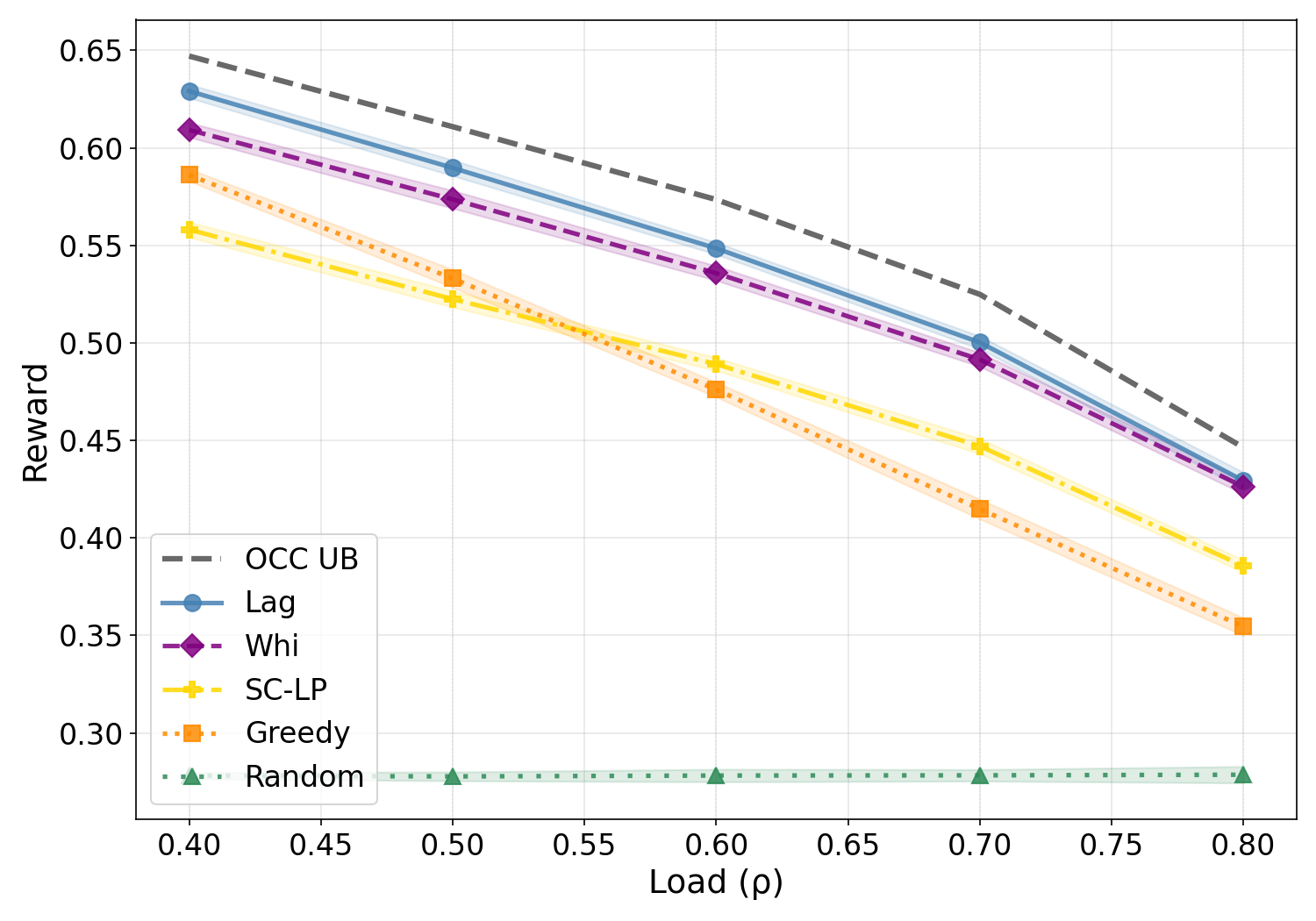 Lag and Whittle both obtain up to 20% higher total similarity than Greedy at intermediate loads.
An Example Where Greedy Struggles
Consider a hypothetical example similar to our running example, with 3 reviewers and 2 types of papers. Except here, we have “Good” papers and “Bad” papers. The two Beginner reviewers always score 0. The Expert scores 1 on the Good papers and 0.01 on Bad papers. Greedy greedily assigns Expert when a Bad paper arrives, when it should clearly save them for a Good paper. In this example, Lag and Whittle both make optimal assignments.
What Greedy does.
What Optimal does.
In this example, we gain 60% improvement over Greedy. When some of the problem parameters are scaled, this improvement can become arbitrarily large.
An Example Where Whittle Struggles
We consider another larger hypothetical example, where some papers and some reviewers uniformly dominate others. A small example:
| LowRank | Expert | Intermediate | Beginner |
|---|---|---|---|
| Good (p=0.5) | 1 | 0.5 | 0 |
| Bad (p=0.5) | 0.5 | 0.25 | 0 |
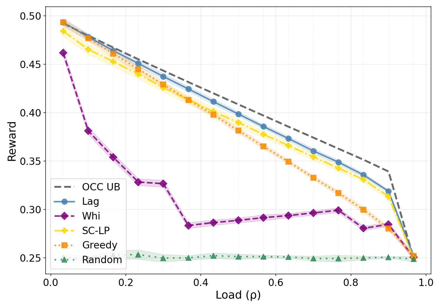
In this example, the optimal fees for the Good and Bad papers are very different and Whittle struggles. Notice that this similarity score matrix is rank $1$. Scaling up the number of reviewers and paper types while keeping the matrix rank 1, Whittle can do 44% worse than even Greedy! Lag still beats all policies.
Why should people care about these results
To me, the most interesting part is that both Lag’s performance and the LP upper bound are close to tight even without the limiting regime in which we can provide optimality guarantees. It also does well on practical examples. If automated journal reviewer assignment deployed a Lag-like policy which accounts for opportunity cost instead of Greedy ( Zhang et al., 2022 ), we may get better matches and thus higher quality reviews.
The framework also extends naturally to many other settings: cab-rider matching, crowdsourcing task-worker assignment, patient-doctor routing. Prior work in this area tends to optimize for competitive ratio — worst-case performance against an adversarial sequence — which can produce algorithms that hedge in ways that hurt expected performance on realistic inputs. Framing the problem as expected reward maximization with a known arrival distribution gives strong numerical performance.
An important limitation in this approach is that Lag requires solving an LP with $V\times R$ variables and constraints. This can become expensive at the scale of large reviewer assignment systems. Whittle sidesteps this: its index has a closed form and scales to large $V$ without any LP solve. On most instances Whittle tracks Lag closely, though the low-rank example shows it can fail when scores are highly correlated across reviewers.
Choosing between them in practice involves this tradeoff. Beyond scalability, the model assumes stationary and known arrival distributions, fixed review durations, and no conflict-of-interest constraints or reviewer bidding — all things a deployed system would need to handle.
