Prediction of Pedestrian Trajectories
People
Description

The objective of this research is to develop algorithms for behavior prediction in dynamic environments. The key short-term objective is to extend our fundamental approach based on max entropy estimation from environments with limited spatial extents, such as indoor environments, to open environments with "infinite horizons" as would be the case in UGV scenarios. The second short-term objective is to study a more general version of the underlying theoretical framework and to develop a plan to mesh it with representations consistent with the needs of planning algorithms.
2. General Progress
We have created the base implementation of the prediction algorithm (see Ref.). This version has been tested using several experimental robotic vehicles. Although the algorithm can take inputs from different sensor types, in particular we have tested using LADAR line scanners as the main sensor. The system produces a display of the map (points and/or occupancy grid), and the positions of the vehicle and detected pedestrians. Furthermore, it is possible to display the prediction of future visitation counts and the distribution of potential destinations together using a transparent overlay. An example of this visualization is illustrated in Figure 1, showing the prediction results as the vehicle traverses the environment. In the occupancy grid map, obstacles are colored in black, while the insert in the lower left corner shows, at a smaller scale, the points map and the vehicle's position. Also shown are the destination density and the prediction of future visitation counts.

Basic prediction from a moving vehicle
A sample experiment is illustrated in the following figure, where a set of four snapshots collected at times t1 through t4 is shown. Without any previous data (i.e. map, destinations, or training trajectories), the vehicle follows a pedestrian and predicts its trajectory. The complete map is shown in the insert as it is being built, while the occupancy map of the subregion surrounding the vehicle is shown in black. The identification of entrances or exits on the border of the subregion is done as the vehicle traverses the environment. The algorithm looks for obstacle-free gaps on each of the four sides of the subregion. If a gap is wide enough for a normal person to go through it, a potential destination is marked at the center of the gap, and added to the list of potential goals. At times t1 and t2 there is one potential goal identified at the top of the figure, as indicated as the brighter red spot. At times t3 and t4 there is also a second potential goal identified at the bottom of the subregion. However, given the starting position of the pedestrian (marked in green), and its current position (marked in red), the algorithm correctly predicts that the pedestrian most likely is heading towards the goal at the top of the subregion, as indicated by the colors of the future visitation count map.

Additional features
The reward (i.e. inverse cost) function used for the example above was learned from a set of training data, and selected as the one that best explains the demonstrated behavior of a pedestrian in the presence of obstacles. This reward function uses a set of six features. The first feature is a constant feature for every grid cell in the environment. The remaining functions are an indicator function for whether an obstacle exists in a particular grid cell, and four "blurs" of obstacle occupancies. To study the issues involved in the incorporation of additional cues from the scene, we have augmented the initial set of obstacle-related features. We have conducted experiments using long walls as environmental features that can influence pedestrian behavior. We trained with a set where pedestrians tended to walk alongside long walls, as opposed to the regular obstacle avoidance maneuvers used to train the initial set. This is illustrated in the following figure. The initial obstacle-related feature set rewards open areas more highly than those closer to obstacles, as seen on the left figure. When a pedestrian tends to walk alongside long walls, the areas closer to them are more highly rewarded, as seen on the right figure. As expected, the resulting predictions reflect this behavior, as shown in Figure 5. Using only obstacle features, the predicted trajectories favor a safe path that maximizes the distance to obstacles, while the augmented set regards trajectories closer to long walls.

Motion cues
For the algorithms developed initially, the generation of goals was done by combining any previous knowledge of goal locations, together with the identification of entrances or exits on the border of the map of the area surrounding the vehicle. This procedure is carried out as the vehicle traverses the environment. However, many potential goals are missed using this approach, since not all of them are found on the borders. For example, consider the scenario shown in the next figure, where the robot is parked across from the entrance of a store. The corresponding map of the area surrounding the robot is shown on the right side, where also a couple of goals identified on the left border of the map are clearly seen. Several potential destinations can be identified in the area shown in the picture on the left: the entrance to the store, the trash can, and the kiosks. Unfortunately, since these locations are not on the border of the map of the vicinity of the robot, they are not marked as goals, and consequently are not considered by the prediction algorithm.
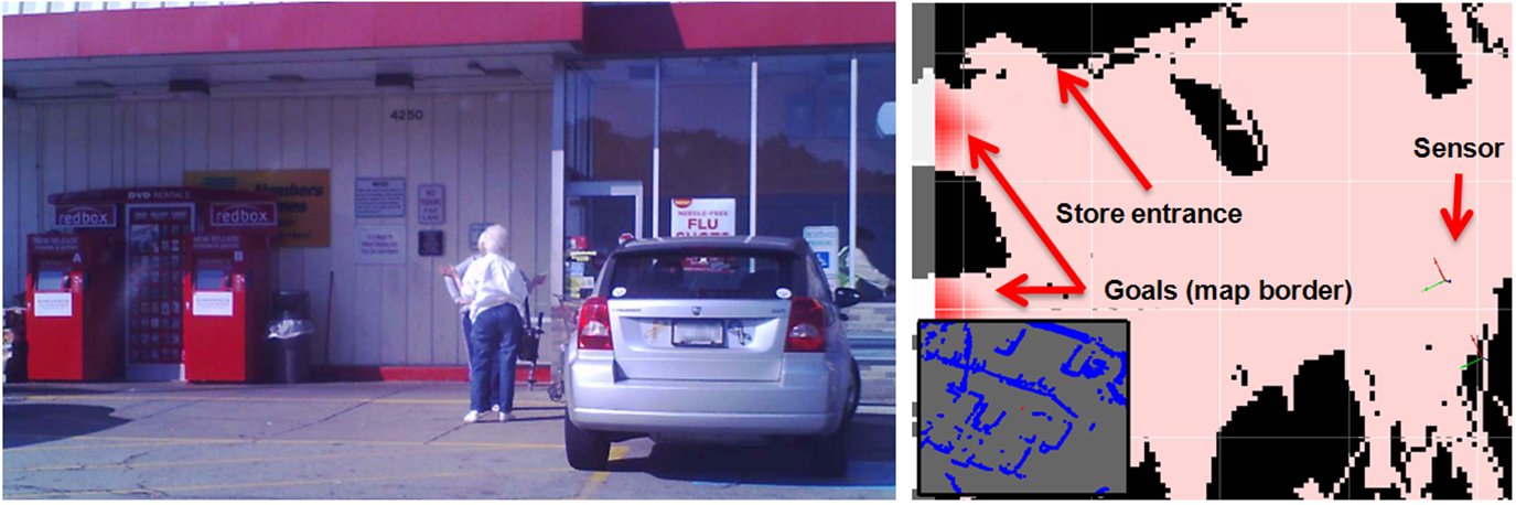
To overcome this limitation, additional cues must be used. Our longer term goal is to use the output of other scene understanding algorithms as input to the prediction algorithm. In the mean time, we started to analyze the motion of every pedestrian to extract additional cues that could represent directional goals. The underlying principle is that pedestrians usually move towards predetermined goals and therefore, a distribution over goals can be obtained from the set of endpoints of each trajectory. We modified the goal generation algorithm to identify a set of conditions as each pedestrian is being tracked. The first condition is when a pedestrian has remained within a certain location for a determined amount of time. The second condition is when a pedestrian's track "disappears" from the sensor's view and seemingly enters an area of the map that is likely to be occupied by an obstacle. The first condition allows the identification of locations where people tend to hover around, which may constitute points of interest and therefore potential goals. The second condition aims to identify locations where people are heading for, despite the current level of knowledge accumulated by the local map. It is reasonable to assume that people will not move towards an area labeled as an obstacle without stopping or slowing down.
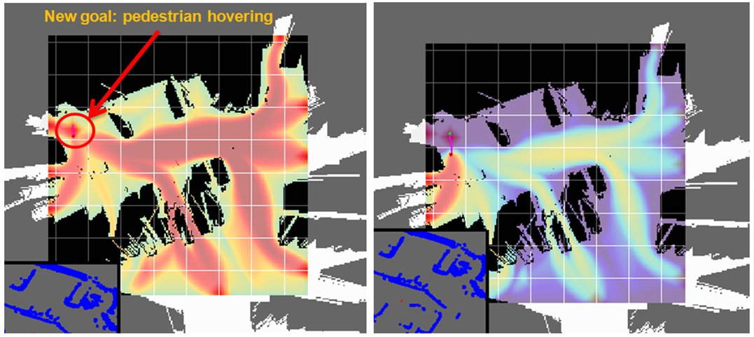
Using these motion cues, the algorithm is capable of identifying directional goals that were missed using the previous approach. In the next figure, a pedestrian remained at the same location for about 5 sec. and then started to walk towards the left. The scenario is the same as described before: the robot is parked across from the entrance of a local store (see previous figure). The pictures show predictions for that pedestrian. A set of potential destinations are identified on the borders of the subregion (colored). Note that a destination was also added inside the subregion, where a pedestrian was standing without moving for a certain amount of time. This is the diamond-like shape located where the track shown started.
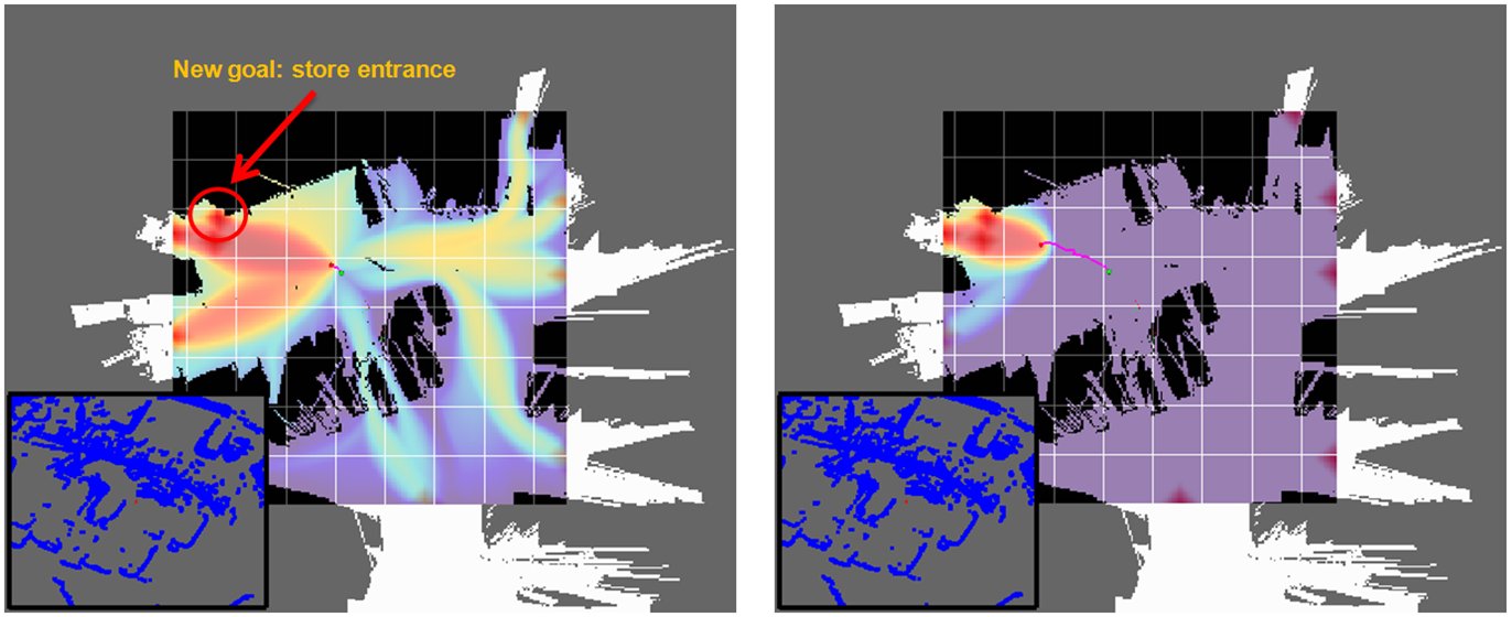
In the following figure, a subsequent step of the experimental run shown before is presented. Note that the goal identified from the hovering pedestrian is now also included inside the subregion. In this case, a new destination was marked at the location where a pedestrian track disappeared. This location is in fact the entrance to the store. This is the diamond-like shape indicated in the left figure. Also note that the map is slightly different, since a car previously parked next to the entrance has left the lot. As shown in the figure, subsequent predictions now incorporate these goals.
3. Current Work
We are currently in the process of evaluating the ability of these algorithms to accurately predict trajectories. We are also investigating ways to implement these algorithms efficiently. Finally, we continue to work towards cloosing the loop by feeding predictions of pedestrian trajectories to planning algorithms.
Reference
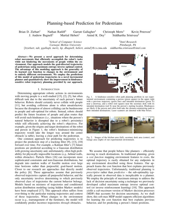
- Planning-based Prediction for Pedestrians
Brian D. Ziebart, Nathan Ratliff, Garratt Gallagher, Christoph Mertz, Kevin Peterson, J. Andrew (Drew) Bagnell, Martial Hebert, Anind Dey, and Siddhartha Srinivasa.
Proc. IROS 2009, October, 2009.
[Paper (PDF)], [BibTeX]
 |
| Paper |
Funding
- Collaborative Technology Alliance Program, Cooperative Agreement W911NF-10-2-0016