Markov localization addresses the problem of state estimation from sensor data. Markov localization is a probabilistic algorithm: Instead of maintaining a single hypothesis as to where in the world a robot might be, Markov localization maintains a probability distribution over the space of all such hypotheses. The probabilistic representation allows it to weigh these different hypotheses in a mathematically sound way.
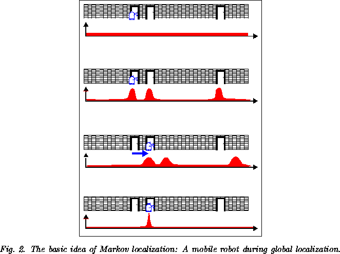
Before we delve into mathematical detail, let us illustrate the basic concepts with a simple example. Consider the environment depicted in Figure 2. For the sake of simplicity, let us assume that the space of robot positions is one-dimensional, that is, the robot can only move horizontally (it may not rotate). Now suppose the robot is placed somewhere in this environment, but it is not told its location. Markov localization represents this state of uncertainty by a uniform distribution over all positions, as shown by the graph in the first diagram in Figure 2. Now let us assume the robot queries its sensors and finds out that it is next to a door. Markov localization modifies the belief by raising the probability for places next to doors, and lowering it anywhere else. This is illustrated in the second diagram in Figure 2. Notice that the resulting belief is multi-modal, reflecting the fact that the available information is insufficient for global localization. Notice also that places not next to a door still possess non-zero probability. This is because sensor readings are noisy, and a single sight of a door is typically insufficient to exclude the possibility of not being next to a door.
Now let us assume the robot moves a meter forward. Markov localization incorporates this information by shifting the belief distribution accordingly, as visualized in the third diagram in Figure 2. To account for the inherent noise in robot motion, which inevitably leads to a loss of information, the new belief is smoother (and less certain) than the previous one. Finally, let us assume the robot senses a second time, and again it finds itself next to a door. Now this observation is multiplied into the current (non-uniform) belief, which leads to the final belief shown at the last diagram in Figure 2. At this point in time, most of the probability is centered around a single location. The robot is now quite certain about its position.