The selective update scheme is based on the observation that during global localization, the certainty of the position estimation permanently increases and the density quickly concentrates on the grid cells representing the true position of the robot. The probability of the other grid cells decreases during localization and the key idea of our optimization is to exclude unlikely cells from being updated.
For this purpose, we introduce a threshold![]()
![]() and update only those grid
cells l with
and update only those grid
cells l with ![]() . To allow for such a
selective update while still maintaining a density over the
entire state space, we approximate
. To allow for such a
selective update while still maintaining a density over the
entire state space, we approximate ![]() for cells
with
for cells
with ![]() by the a priori
probability of measuring
by the a priori
probability of measuring ![]() . This quantity, which we call
. This quantity, which we call
![]() , is determined by averaging over all possible
locations of the robot:
, is determined by averaging over all possible
locations of the robot:
Please note that ![]() is independent of the current
belief state of the robot and can be determined beforehand. The
incremental update rule for a new sensor measurement
is independent of the current
belief state of the robot and can be determined beforehand. The
incremental update rule for a new sensor measurement ![]() is changed
as follows (compare Equation (9)):
is changed
as follows (compare Equation (9)):
By multiplying ![]() into the normalization factor
into the normalization factor
![]() , we can rewrite this equation as
, we can rewrite this equation as
where ![]() .
.
The key advantage of the selective update scheme given in
Equation (39) is that all cells with ![]() are updated with the same value
are updated with the same value ![]() .
In order to obtain smooth transitions between global localization and
position tracking and to focus the computation on the important
regions of the state space L, for example, in the case of
ambiguities we use a partitioning of the state space. Suppose the
state space L is partitioned into n segments or parts
.
In order to obtain smooth transitions between global localization and
position tracking and to focus the computation on the important
regions of the state space L, for example, in the case of
ambiguities we use a partitioning of the state space. Suppose the
state space L is partitioned into n segments or parts ![]() . A segment
. A segment ![]() is called active at time t
if it contains locations with probability above the threshold
is called active at time t
if it contains locations with probability above the threshold
![]() ; otherwise we call such a part passive because
the probabilities of all cells are below the threshold. Obviously, we
can keep track of the individual probabilities within a passive part
; otherwise we call such a part passive because
the probabilities of all cells are below the threshold. Obviously, we
can keep track of the individual probabilities within a passive part
![]() by accumulating the normalization factors
by accumulating the normalization factors ![]() into a value
into a value ![]() . Whenever a segment
. Whenever a segment ![]() becomes passive,
i.e. the probabilities of all locations within
becomes passive,
i.e. the probabilities of all locations within ![]() no longer
exceed
no longer
exceed ![]() , the normalizer
, the normalizer ![]() is initialized to
1 and subsequently updated as follows:
is initialized to
1 and subsequently updated as follows: ![]() . As soon as a part becomes active
again, we can restore the probabilities of the individual grid cells
by multiplying the probabilities of each cell with the accumulated
normalizer
. As soon as a part becomes active
again, we can restore the probabilities of the individual grid cells
by multiplying the probabilities of each cell with the accumulated
normalizer ![]() .
By keeping track of the robot motion since a part became passive, it
suffices to incorporate the accumulated motion whenever the part
becomes active again. In order to efficiently detect whether a
passive part has to be activated again, we store the maximal
probability
.
By keeping track of the robot motion since a part became passive, it
suffices to incorporate the accumulated motion whenever the part
becomes active again. In order to efficiently detect whether a
passive part has to be activated again, we store the maximal
probability ![]() of all cells in the part at the time it
becomes passive. Whenever
of all cells in the part at the time it
becomes passive. Whenever ![]() exceeds
exceeds
![]() , the part
, the part ![]() is activated again because it contains at
least one position with probability above the threshold.
In our current implementation we partition the state space L such
that each part
is activated again because it contains at
least one position with probability above the threshold.
In our current implementation we partition the state space L such
that each part ![]() consists of all locations with equal
orientation relative to the robot's start location.
consists of all locations with equal
orientation relative to the robot's start location.
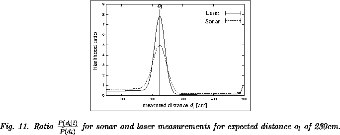
To illustrate the effect of this selective update scheme, let us
compare the update of active and passive cells on incoming sensor
data. According to Equation (39), the difference lies
in the ratio ![]() . An example of this ratio
for our model of proximity sensors is depicted in
Figure 11 (here, we replaced
. An example of this ratio
for our model of proximity sensors is depicted in
Figure 11 (here, we replaced ![]() by a
proximity measurement
by a
proximity measurement ![]() ).
).
In the beginning of the localization process, all cells are active and
updated according to the ratio depicted in
Figure 11. The measured and expected
distances for cells that do not represent the true location of the
robot usually deviate significantly. Thus, the probabilities of these
cells quickly fall below the threshold ![]() .
.
Now the effect of the selective update scheme becomes obvious: Those
parts of the state space that do not align well with the orientation
of the environment, quickly become passive as the robot localizes
itself. Consequently, only a small fraction of the state space has to
be updated as soon as the robot has correctly determined its position. If,
however, the position of the robot is lost, then the likelihood ratios
for the distances measured at the active locations become smaller than
one on average. Thus the probabilities of the active locations
decrease while the normalizers ![]() of the passive parts increase
until these segments are activated again. Once the true position of
the robot is among the active locations, the robot is able to
re-establish the correct belief.
of the passive parts increase
until these segments are activated again. Once the true position of
the robot is among the active locations, the robot is able to
re-establish the correct belief.
In extensive experimental tests we did not observe evidence that the selective update scheme has a noticably negative impact on the robot's behavior. In contrast, it turned out to be highly effective, since in practice only a small fraction (generally less than 5%) of the state space has to be updated once the position of the robot has been determined correctly, and the probabilities of the active locations generally sum up to at least 0.99. Thus, the selective update scheme automatically adapts the computation time required to update the belief to the certainty of the robot. This way, our system is able to efficiently track the position of a robot once its position has been determined. Additionally, Markov localization keeps the ability to detect localization failures and to relocalize the robot. The only disadvantage lies in the fixed representation of the grid which has the undesirable effect that the memory requirement in our current implementation stays constant even if only a minor part of the state space is updated. In this context we would like to mention that recently promising techniques have been presented to overcome this disadvantage by applying alternative and dynamic representations of the state space [Burgard et al. 1998b, Fox et al. 1999].