Fast Image-Based Tracking
by Selective Pixel Integration

Frank Dellaert and Robert Collins
Computer Science Department and Robotics Institute
Carnegie Mellon University
Pittsburgh PA 15213

Abstract

We provide a fast algorithm to perform image-based tracking, which relies on the selective integration of a small subset of pixels that contain a lot of information about the state variables to be estimated. The resulting dramatic decrease in the number of pixels to process results in a substantial speedup of the basic tracking algorithm. We have used this new method within a surveillance application, where it will enable new capabilities of the system, i.e. real-time, dynamic background subtraction from a panning and tilting camera.

1. Introduction/Philosophical Approach

One of the fundamental tasks of real-time processing has been image-based tracking through a video sequence using a parametric motion model. This includes both tracking of a moving object through an image sequence [5] as well as registering of whole images to a reference view to provide software video stabilization [2,8].

Figure 1. Selective pixel integration selects pixels with a high information content with respect to the variables to be estimated. In this image, the pixels marked in white are informative with respect to pan, tilt and roll of the camera (click on the image to enlarge).

In this paper we will provide a fast algorithm to perform image-based tracking, based upon the following observation:

Using only a small percentage of the available pixels, selected on their information content with respect to the state variables, yields a tracking algorithm that is as accurate as conventional tracking algorithms that use entire images or image pyramids, yet orders of magnitude faster.

This observation relies on the fact that only very few pixels actually contribute towards the shaping of the error function that is minimized (see Figure 1). In the case of tracking, this is typically a weighted sum of square errors dependent on the parameters to be estimated. In the neighborhood of the minimum, the shape of the error function is governed by its Hessian. When inspected, the vast majority of pixels are seen to contribute little or nothing to the value of the Hessian, suggesting that these pixels can be safely ignored for the purpose of tracking.

Selective pixel integration is not yet another feature selection algorithm: we are truly selecting pixels, not small feature windows. Feature-based methods track the location of a small feature window, and the x-y coordinate of the feature is provided as input to the estimation method. In our case, we look directly at the value of a particular pixel. Each pixel will change in a predictable way as a function of the parameters, and thus each pixel in isolation provides some information on each of the parameters that cause it to change its value. The amount of information provided can be rigorously computed, as will be shown below. Based on this computed information content, we can designate some pixels as being better than others for estimating state variable updates.

2. Selective Pixel Integration

2.1 Definition and Example of Tracking

Figure 2. An example of a tracking problem is to estimate, over time, the parameters X=[a b c d e f g h]' that warp the template T to the changing input image I, according to a 2D projective transformation (a 2D homography).

We will define tracking as estimating the transformation between a reference image or template T and the current input image I over time. Let's define the state X and the measurement function h(X,T) that together specify this transformation. An example we will use throughout is the case where h is a projective warp of the template T, and X contains as components the eight independent parameters that are needed to specify the projective warp. The situation is illustrated in Figure 2.

The application we discuss below (as well as the example in Figure 2) involves whole images and is therefore more often referred to as image registration, but the algorithm we discuss is in no way limited to this type of application. Please refer to [6,5,4,3] for other examples of image based tracking, in particular face tracking, tracking of planar objects in 3D, and estimating lighting changes as well as deformations of shape. [5] also talks about how one can deal with outliers and occlusion, which we will not discuss in detail here.

2.2 A General Tracking Algorithm

The most often used method to find an estimate for X at each time step is minimizing the sum of square errors:

$$X^* = \mathop{\rm argmin \,}_{X} (I-h(X,T))^2$$ (1)

where we have used e² as shorthand for e'e, and where e'denotes the transpose of a matrix or vector e. This can be solved using the pseudo-inverse:

X^* - X₀ = (H' H)^-1H' (I-h(X,T)) (2)

where X₀ is a prediction based on the previous tracking history, and H is the measurement Jacobian. It is defined as the Jacobian matrix of h(.,.) with respect to X, and evaluated at X₀. If h is non-linear, more than one iteration might be required to converge to the minimum.

2.2.1 The interpretation of the Measurement Jacobian

Figure 3. Jacobian images show how pixel values will change with respect to a change in state variables. An example image and its Jacobian images with respect to (in reading order) incremental camera roll, pan and tilt. Red and green are decrease and increase in pixel value, respectively. Intuitively, a change and pan and tilt will cause most change at vertical and horizontal edges, respectively. An equal amount of roll causes much less change in the image, with most change occurring at the edges and none in the middle of the image.

The measurement Jacobian has an intuitive explanation in terms of Jacobian images [4,3], which are a pictorial representation of how a pixel's value will change with respect to a change in state variables. They are simply the columns H_j of the measurement Jacobian H, reordered as images. Hager [6,5] calls these images 'motion templates'. An example is shown in Figure 3.

It is clear that these Jacobian images, and thus H, are in general a function of the state X. Furthermore, they are expensive to compute, as each one of them is an image of the same size as the original template image. However, now there are n of them, where n is the dimension of X. Furthermore, they are in general non-linear and complex functions of the state and the template, as they are computed as the point-wise multiplication of induced flow fields and the template gradient images [3,5]. More about the computation of Jacobian images appears in the Appendix.

2.2.2 Computational Demands

The solution outlined above works, but is expensive, as hinted at in the previous paragraph. At each time step, and this possibly for multiple iterations, we need to compute (a) the Jacobian images H_j, (b) the pseudo-inverse (H' H)^-1 H', and (c) we need to warp the template T according to the changing estimate of X.

One trick to reduce the computation is to warp the image I towards the template T instead, and minimize an approximate criterion:

$$dX^* = \mathop{\rm argmin \,}_{dX} (h(X_0^{-1},I)-h(dX,T))^2$$ (3)

where h(X₀^-1,I) informally denotes the inverse warp corresponding to h(X₀,T). We now look for the best residual warp h(dX,T) that accounts for the difference between the warped image h(X₀^-1,I) and the template T. We then update the state estimate X₀ using this incremental state update dX^*:

$$X^* = X_0 \oplus dX^*$$ (4)

with $\oplus$ denoting the update operation. The update might be a simple addition, as in the case of pure translation, or matrix multiplication, when composing general projective transformations.

Again, using the pseudo-inverse, we get an expression for dX^*:

dX^* = (H' H)^-1 H' (h(X₀^-1,I)-T) (5)

where our initial guess for dX is 0, i.e. we assume X₀ is correct, and h(0,T)=T. This trick makes it possible to pre-compute the Jacobian H, as we will always take 0 as the initial guess for dX, and so the Jacobian is evaluated only at 0. Thus, the pseudo-inverse of H can also be pre-computed [5].

2.2.3 Gaussian Pyramids

Although precomputing H saves a lot of computation, we still need to warp the image I at each time step, possibly multiple times if we need to iterate due to a non-linear h. Especially if I is large, e.g. complete images, this can be prohibitively expensive. One way to deal with this is to down-sample the images into a Gaussian pyramid. In many image registration applications enough accuracy can be obtained by only registering the low-resolution versions of I and T, and the cost of warping is not that high, as there are less pixels in the downsampled images. However, we still need to do the work of filtering and down-sampling to obtain the pyramid.

2.3 Selective Pixel Integration

A completely different approach is selective pixel integration, i.e. looking at the pixels in the original images that yields the most information about dX. Intuitively, a pixel in a non-textured, flat area does not contribute much, if anything. Also, pixels that suffer from the aperture problem only contribute knowledge about part of the state. If we could find a small subset of the pixels that yield enough information about the state to satisfy our demands on accuracy, we could dramatically reduce the cost of warping, and thereby the overall cost of tracking, without downsampling.

It turns out that a similar question has been asked before in the MRI community [10]: suppose we can shoot any of thousands of rays at a person to get an MRI image reconstruction, but we want to use as few rays as possible, which ones should we choose ? In both cases, the underlying question is the same:Which measurements yield the most information about the quantity to be estimated ?

2.3.1 The 'Best Pixel'

Suppose we could only look at one pixel, which pixel should we pick ? First, one pixel might yield only partial information about the state X. The answer will thus depend on what we already know. In addition, the matrix H'H in the pseudo-inverse will become singular in this case, as the measurement Jacobian H will be rank deficient. Both reasons prompt us to introduce prior knowledge.

Figure 4. The images above show the decrease in uncertainty resulting from looking at one pixel only. The actual quantity shown is the decrease in the trace of the state covariance matrix, relative to the prior information P. The brighter a pixel, the more information it provides. This heavily depends on our prior knowledge: at the left, the only uncertain state variable is the roll of the camera with respect to the template. In the image at the right, roll is known, but pan and tilt are not known precisely (up to one degree).

Let us assume that we can characterize our prior knowledge about dXby a Gaussian, centered around 0 and with covariance matrix P. We also need to know something about the measurement itself: how trustworthy is it? If we assume that the pixels are contaminated by i.i.d. zero-mean Gaussian noise, this information is specified by the variance $\sigma^2$. The maximum a posteriori or MAP estimate for dX, given one pixel j, is then found by minimizing a criterion which now takes into account the deviation of dX from 0:

$$dX^* = \mathop{\rm argmin \,}_{dX} \sigma^{-2} (h_i(X_0^{-1},I)-h_i(dX,T))^2 + dX' P^{-1} dX$$ (6)

where h_i is the ith component of h, i.e. the recipe to warp one pixel according to X. This is done by (repeatedly, if needed) solving the linear system of normal equations, with H_i the ith row of the Jacobian H:

$$(\sigma^{-2} H_i' H_i + P^{-1}) dX^* = \sigma^{-2} H_i' (h(X_0^{-1},I)-T)$$ (7)

It is known from estimation theory that after convergence, the posterior distribution P(dX|I) (our full knowledge about dX) can be locally approximated as a Gaussian with covariance equal to the inverse of the Hessian Q:

$$P^+ = (\sigma^{-2} H_i' H_i + P^{-1})^{-1} = Q^{-1}$$ (8)

To find the best pixel, we would like to minimize this uncertainty. Although P⁺ is an $n \times n$ matrix (where n is the dimension of the state X), the trace of P⁺ is also a meaningful quantity: it is equal to the expected variance of the error function after we obtained dX^*. Thus, one way to find the best pixel i is to minimize the trace of P⁺ [10]:

$$i = \mathop{\rm argmin \,}_{i} \mathop{Tr} \, (\sigma^{-2} H_i' H_i + P^{-1})^{-1}$$ (9)

Note that the identity of the best pixel is highly dependent on the prior knowledge P and on the form of h. In Figure 4, this is illustrated graphically for varying prior knowledge P. More examples of this dependence on P can be found here. Note also that all this can be generalized to arbitrary noise covariance matrices R, so that correlated noise can be modeled equally well.

2.3.2 The Best Subset of Pixels

Finding the best pixel is easy, but what about the best subset of pixels? It turns out this question is hard. Intuitively, the best pixel and the second best pixel do not necessarily constitute the best set of two pixels, as they might provide redundant information. In fact, the 'best pixel' might not even be a member of the best 2-set at all. in general, the only way the find the optimal set of M pixels, is to look at all possible subsets of size M within the m pixels. But this is a combinatorial search problem of immense proportions, as there are binomial(M m) such sets. With m on the order of 10⁶ and M on the order 10², this is infeasible.

Figure 5. An example of selecting the subset of the best 1000 pixels in an image using the greedy SFS algorithm as described in \cite{Reeves95}. At the left, the set of 1000 pixels for known roll but unknown (incremental) pan and tilt. The color indicates the order in which pixels were selected by SFS, brighter meaning earlier in the sequence. As can be seen, mostly pixels on diagonal edges are picked out, as these provide information both on pan and on tilt. At the right, a set of 1000 pixels when pre-whitening is applied to remove spatial correlation.

A greedy algorithm was given in [10], based on a feature selection algorithm from machine learning, sequential forward search (SFS). In this algorithm, a list of pixels is created greedily. The procedure starts with a list containing only the best pixel, optimal in conjunction with the prior information P. The integration of this pixel gives a new covariance matrix, B, which now combines the information in P and the best pixel. Then, the best pixel is found that provides the most information relative to B. This process is repeated until M pixels are found.

We have implemented Reeves' SFS algorithm, and an example is shown in Figure 5. One problem that tends to arise, however, is that the selected pixels tend to cluster in the image, which would lead to non-robust tracking behavior in case of correlated noise such as occlusion, lens smudges etc... To remedy this, we have also applied pre-whitening to the Jacobian to cope with spatially correlated noise. The details are beyond the scope of this paper, but the effect is very noticeable. In the right panel of Figure 5, the new set of pixels obtained after pre-whitening is much more spread out, which is what we want.

2.3.3 Random Pixel Selection

For all the theoretical merit of Reeves' SFS algorithm, we have found that an even simpler algorithm provides more robustness in the case of image based tracking. Even the pre-whitened version of SFS still clusters pixels in a few regions of the image, which leads to instabilities in the tracking process in the case of occlusion. The answer we came up with is simple but works: we simply select M pixels randomly from the top 20 percent of the 'best' pixels. In other words, we compute an image like the one in Figure 4, sort the pixels according to information content (with respect to a prior), drop the bottom 80 percent, and randomly select M pixels from the remaining set. Examples of sets of pixels thus obtained are shown below in the application section.We have found that this simple method performs quite well in practice, and it is also straightforward to implement.

At the time of writing, we are also experimenting with an alternative method (also used by Zhang in a different context), that imposes an imaginary grid on the image, then select the M/N best pixels from each grid cell, where N is the number of grid cells. This forces the selections to be spread evenly over the whole image. For the selection within a cell, we again resort to Reeves' SFS. We are evaluating whether this method allows us to further reduce the overall number of pixels needed to accurately track.

2.3.4 The Selective Pixel Integration Tracker

The final tracking algorithm looks as follows:

1.

Pre-compute the Jacobian images H for dX=0.

2.

Pick a canonical prior knowledge covariance matrix P, and pixel noise covariance $\sigma^2$.

3.

Select the M best pixels for the template T, relative to P.

4.

For each time step:

(a)

Predict the state X₀ using a model for the dynamics.

(b)

Inverse warp the M selected pixels to the template,
$z_i=h_i(X_0^{-1},I), i\in \{1..M\}$

(c)

Calculate the error
$e_i = z_i-T(m_i), i\in \{1..M\}$

(d)

Find the best dX^* by solving $(\sigma^{-2} H_M' H_M + P^{-1}) dX^* = \sigma^{-2} H_M' e$
where H_M is the part of H corresponding to the M selected pixels.

(e)

Calculate $X^* = X_0 \oplus dX^*$

(f)

Iterate if necessary

Most of the computation is now done off-line, and none of the on-line computation involves more than M pixels. The most expensive operations are the warp of the M pixels, and the computation of the Hessian $Q = \sigma^{-2} H_M' H_M + P^{-1}$. The latter can also be precomputed if it can be guaranteed that all M pixels will be within the region to which I has been warped. If this is not the case, one can still save on computation by precomputing H_M' H_M, and subtracting the contribution for the relatively few pixels that fall outside the valid set.

3. Discussion: Implications and Limitations

The implications of our new method are potentially far-reaching. Since we can dramatically reduce the amount of computation spent on tracking, the CPU is freed to do other tasks that might otherwise have been impossible to do within real-time constraints. In the next section we will present the outline of this within a surveillance application.

In addition, we can increase the rate at which frames can be processed. Paradoxically, many tasks actually become easier to do at higher rates, e.g. frame or field rate, as the image displacements become smaller and easier to track over time, and we can use simpler motion models while still accurately predicting what we should see in the next frame.

Finally, selective pixel integration provides an alternative to downsampling by working directly with the image pixels, and reasoning about what each individual pixel can tell us about the state variables.

It is also important to understand the limitations of this method. Most importantly, it will only work in a relatively small neighborhood around the true local minimum, as it depends crucially on the validity of the Jacobian H. Further away from the minimum, at best the algorithm will have to iterate multiple times, at worst it will diverge entirely. We feel, however, that this is not a significant limitation, as accurate predictions is always a hallmark of real-time applications: the better the prediction, the less computation needs to be expended.

There also a question of robustness: we have already remarked that the theoretically suporior method of Reeves' greedy selection scheme suffers from robustness problems when used with image based tracking. The random selection method works quite well in our example application (see below), but might integrate more pixel than strictly necessary. Indeed, in theory, 10 or 20 pixels should suffice to track, and we do indeed see that happen with synthetic sequences. More work is needed in the case of real images, though, to understand and model the noise and bring the number of pixels down even further.

4. Application: Real-Time Pan-tilt Tracking for VSAM

4.1 Motivation

The problem we address in this section is the detection of object motion from a continuously panning and tilting video camera. Over the past two years there has been a great deal of computer vision research devoted to automated video surveillance and monitoring (VSAM) [7]. A low-level task that is common to all video surveillance systems is to automatically detect moving objects (people and vehicles), and to track them as they move through the scene. Pan-tilt camera platforms can maximize the virtual field of view of a single camera without the loss of resolution that accompanies a wide-angle lens, and allows for active tracking of an object of interest through the scene.

Automatic detection of moving objects from a stationary video camera is easy, since simple methods such as adaptive background subtraction or frame differencing work well. These methods are not directly applicable to a camera that is panning and tilting since all image pixels are moving. However, this situation is approximately described as a pure camera rotation, and the apparent motion of pixels depends only on the camera motion, and not at all on the 3D structure of the scene. In this respect, the problem we are addressing is much easier than if the camera were mounted on a moving vehicle traveling through the scene.

At this time, adaptive background subtraction provides motion segmentation results with the least time lag and most complete object boundaries [11,9,13]. The general idea is to maintain statistics about the intensity or color values at each pixel in the image, and to gradually update these statistics over a moving window in time to adapt to lighting variations. Each new image is compared to this 'reference' image, and pixels that deviate significantly from their reference values are flagged as potentially belonging to a new moving object. Object hypotheses are generated by performing connected components on the changed pixels, followed by blob tracking between video frames.

We ultimately seek to generalize the use of adaptive background subtraction to handle panning and tilting cameras, by representing a full spherical background model. There are two algorithmic tasks that need to be performed: 1) background subtraction: as the camera pans and tilts, different parts of the full spherical model are retrieved and subtracted to reveal the independently moving objects. 2) background updating: as the camera revisits various parts of the full field of view, the background intensity statistics in those areas must be updated.

Both tasks defined above, background subtraction and background updating, depend on knowing the precise pointing direction of the sensor, or in other words, the mapping between pixels in the current image and corresponding 'pixels' in the background model. Although we can read the current pan and tilt angles from encoders on the pan-tilt mechanism, this information is only reliable when the camera is stationary. Due to unpredictable communication delays, we can not precisely know the pan-tilt readings for a given image while the camera is moving. Our solution to this problem is to register the images to the current background model in order to infer the correct pan-tilt values while the camera is rotating.

4.2 Implementation

4.2.1 Scene Representation

Figure 6. The collection of views that we used in one experiment. There.are 40 views in total, with pan and tilt in the range 40:-20:100 and -4:-10:-44, respectively.The top-left image is the pan=40, tilt=-4 image. (Click on the image for a closer look)

Maintaining a background model larger than the camera's physical field of view entails representing the scene as a collection of images [8]. In our case, an initial background model is collected by methodically collecting a set of images with known pan-tilt settings. An example view set is shown in Figure 6. One approach to building a background model from these images would be to stitch them together into a spherical or cylindrical mosaic [8,12]. We choose instead to use the set of images directly, determining which is the appropriate one to use based on the distance in pan-tilt space. The warping transformation between the current image and a nearby reference image is therefore a simple planar projective transformation, rather than a more time consuming trigonometric mapping to the surface of a sphere or cylinder.

4.2.2 Pixel Selection

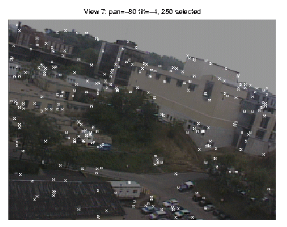
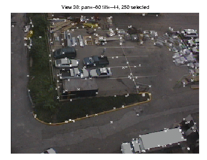
Figure 7. Two example views with the selected pixels. The state variables to be optimized are pan, tilt and roll.

For each of the views, the set of selected pixels for selective pixel integration is pre-computed, using the random selection algorithm outlined above. Two example sets are shown in Figure 7. The canonical prior we used had 1 degree standard deviation on pan and tilt, and 0.1 degrees on roll.

4.2.3 Tracking Pan and Tilt

Our tracking algorithm is described in detail below. For each time step, we:

1.

Predict X₀, the pan, tilt and roll for the input image I, using a motion model (described in detail in the next section).

2.

Select the closest view T (in terms of pan and tilt)

3.

Calculate the approximate homography A^T_I to warp T to I. Since we know the pan and tilt for the view T, the calibration matrix K, and we have an estimate X₀ for the pan, tilt and roll of the current image, we can calculate this homography as
A^T_I = K R_T' R_I K^-1
where R_T is the rotation matrix for the view T, and R_I is the estimated rotation matrix for the input image.

4.

Calculate the homography for the inverse warp, A^I_T = (A^T_I)^-1

5.

Inverse warp the M selected pixels to T, according to A^I_T. For each of the selected pixels m_i, where $i \in \{1..M\}$, we

(a)

Calculate p_i = A^I_T m_i, the corresponding image coordinate according to the projective warp A^I_T.

(b)

If p_i is not within the bounds of I, we discard this selected pixel.

(c)

Resample the image I at that coordinate p_i, obtaining g_i(A^I_T,I), using either a bilinear or Gaussian filter. Here g denotes the projective warp.

(d)

Collect the resulting values in the measurement z
$z_i=g_i(A^I_T,I), i \in \{1..M\}$

(e)

Collect the predicted values into the prediction y
$y_i=T(m_i), i \in \{1..M\}$

(f)

Calculate the error
e_i=z_i-y_i.

6.

Optimize for the best incremental rotation $dX^*=[\omega_x\, \omega_y\, \omega_z]'$, by solving
$(\sigma^{-2} H_M' H_M + P^{-1}) \, dX^* = \sigma^{-2} H_M' e$
where H is the pre-computed Jacobian with respect to incremental pan, tilt and roll (see Figure 3). The measurement function is a projective warp according to incremental pan, tilt and roll, parametrized using the incremental rotation matrix

$$R(dX) = R(\omega_x,\omega_y,\omega_z) = \begin{pmatrix} 1 & ... ...\omega_z& 1 & -\omega_x\\ -\omega_y& \omega_x& 1 \end{pmatrix}$$ (10)

7.

Update the homography A^I_T and calculate X^*. We can do this as
$A^I_T \leftarrow K R(dX^*) K^{-1} A^I_T$
The final estimated rotation matrix for the image I is then obtained by
R_I = R_T K^-1(A^I_T)^-1 K
and $X^*=[pan \, tilt \, roll]'$ can be easily calculated from R_I.

8.

Iterate if necessary

4.2.4 Multiple Model Prediction

A prerequisite for fast tracking and a necessary component to make selective pixel integration work is adequate prediction. The selective pixel integration idea relies on the measurement Jacobian H, which will only be valid within a small window near the actual minimum. In addition, the better the prediction, the less iterations are necessary to converge to the minimum of the non-linear optimization criterion.

Figure 8. A 'ground truth' sequence (see text on how it was obtained) showing the abrupt changes of pan and tilt as a consequence of discontinuous user input, used to steer the camera. Note that a constant velocity model will work fine except at the speed discontinuities, where it fails dramatically.

In our prototype application, we are tracking manually steered pan-tilt movements, which is not an easy case. The camera is controlled by keyboard interaction, using the four arrow keys found on a standard keyboard. Pan is controlled by the horizontal arrows, tilt by the vertical arrows. Since this is essentially binary control, the pan-tilt trajectories change abruptly. During a continuous movement, the tracking is not hard, but coping with the trajectory changes is.

To deal with the problem of abrupt trajectory changes, we implemented a multiple model Kalman filter. The velocity at which the pan and tilt changes is assumed known, but at each timestep there are three different possibilities for pan and tilt: (U)p, (S)ame or (D)own. This makes for 9 different motion models. The implementation closely follows the exposition in [1]. At each time step, we make a prediction X_0j for each model of the 9 models:

$$X_{0j} = X(t-1) + \Omega_j$$ (11)

where $\Omega_j$ contains the hypothesized change in pan and tilt for model j. The likelihood of each model is obtained by warping a severely subsampled version of the image (20 by 15 pixels, indicated by I_s and T_s) to the hypothesized location in the template, and evaluating the sum of squared errors:

E_j = (h(X_0j^-1,I_s)-T_s)² (12)

The likelihood of model j given I_s is then (with $\beta$ a temperature parameter):

$$P(I_s\vert j) = \exp(-0.5 \beta E_j)$$ (13)

The posterior probability for each of the models is calculated based on the most likely model at the previous time step and a matrix of transition probabilities p_ij. See [1] for additional details. After this, the model with the highest posterior probability is chosen for tracking.

4.3 Results

4.3.1 Evaluating Performance

Embedded Quicktime movie of a tracking sequence.

(a) Camera Input

(b) Selected View

(c) Registered image

(d) Difference Image

Figure 9. An embedded Quicktime movie showing a tracking sequence of 300 frames long (click here for downloadable MPEG, AVI, and higher resolution versions). The movie is divided in four panels: (a) The camera input shows what is seen by the camera during panning and tilting. (b) The selected view shows one of the (in this case) 40 input views to which the current image is actively registered. (c) The registered image is the camera input after warping it to the selected view. (d) The difference image shows the difference between (b) and (c).

We have tested this algorithm based on several sequences of 300 frames in length, and consistently obtain tracking rates at about 60 frames per second, when integrating 250 pixels (M=250). This is with quarter size images, obtained by grabbing images from the camera and subsampling them by pure decimation.

To evaluate the performance of the algorithm, we do the frame-grabbing off-line, and store the images in memory. We store the images in memory because of two reasons: first, at the time of writing we only have a prototype system working, which is not yet integrated with our on-line frame-grabbing software. We do not believe the overhead of image and memory I/O will significantly impact the timing results. Second, we our method performs at much higher than frame rates, and when grabbing at a fixed framerate we would have no way to assess the algorithm's performance.

We then run the tracker, and note how long it takes to process all 300 frames. This is always around 5 seconds, with fluctuations because the number of iterations per frame might differ from frame to frame. We are convinced that these preliminary performance figures can yet be improved upon, as part of our research code still runs within MATLAB. We are currently porting the entire algorithm to C++.

Figure 10. Estimated pan, tilt and roll.

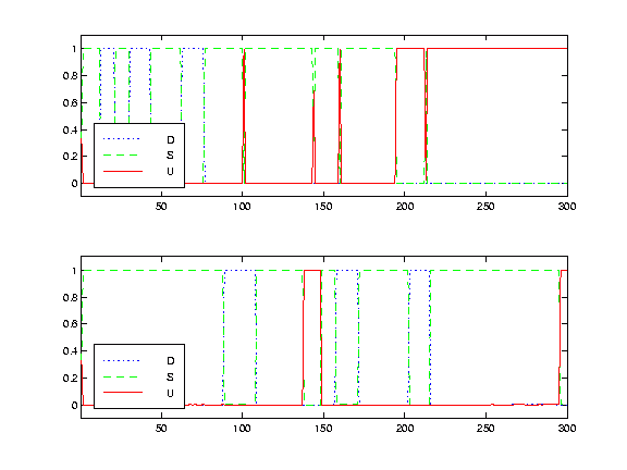
Figure 11. Marginal posterior probabilities for the different motion models. The top panel shows the posterior probability of three different models for pan: (U)p, (S)ame, and (D)own. The bottom panel shows the same for tilt. Note the correspondence with Figure 10.

A video segment recording the tracking of a typical sequence is shown in Figure 9. The measured pan, tilt and roll angles are shown in Figure 10. The posterior probability of each motion model is shown in Figure 11.

4.3.2 Evaluating Tracking Accuracy

Figure 12. Comparison with ground truth.

To evaluate the accuracy of the algorithm, we obtained 'ground truth' by running the tracker using 3-level pyramids of the images and the views, and using all pixels. Because of the hierarchical approach, the initial estimates at higher-resolution levels are very good and high accuracy is obtained. Since we use complete images up to a quarter size, this approach is slow but yields accurate results. The comparison of the estimated pan-tilt-roll angles with the ground truth is shown in Figure 12. Most of the noticeable spikes are associated with shifts between views.

5. Conclusion

We have presented a novel approach to obtaining better-than-frame-rate image-based tracking. It relies on the selective integration of a small subset of pixels that contain a lot of information about the state variables to be estimated. This dramatic decrease in the number of pixels to process results in a substantial speedup of the basic tracking algorithm. We have used this new method within a surveillance application, where it will enable new capabilities of the system, i.e. real-time, dynamic background subtraction from a panning and tilting camera.

   
Appendix: Computing the Jacobian Images

The calculation of the Jacobian images is detailed by Dellaert [4]. Hager & Belhumeur have a similar derivation in [6,5]. Our paper [4] is available on-line:

Jacobian Images of Super-Resolved Texture Maps for Model-Based Motion Estimation and Tracking
F. Dellaert, S. Thrun, and C. Thorpe, IEEE Workshop on Applications of Computer Vision (WACV'98), Princeton, New Jersey, October 19-21, 1998, pp. 2-7.
Download: pdf [262 KB], ps.gz [798 KB] copyrighted

In essence, the calculation amounts to a simple application of the chain rule: the Jacobian H at X₀ is defined as the partial derivative of h with respect to X, evaluated at X₀:

$$H(X_0) = \frac{\partial h(X,T)}{\partial X}\biggr\rvert_{{X_0}}$$ (14)

which is a $m \times n$ matrix, with m is the number of pixels in an image, and n the dimension of the state. One entry H_ij is the partial derivative of pixel h_i(X,T) with respect to state variable X_j:

$$H_{ij}(X_0) = \frac{\partial h_i(X,T)}{\partial X_j}\biggr\rvert_{{X_0}}$$ (15)

If h(.,.) is a warp implemented by simple point sampling, h has the form h_i(X,T) = T(f(p_i,X),T), where f is the coordinate transform that transforms image coordinate p_i accoring to X into an template coordinate m_i=f(p_i,X). It is a $2 \times 1$ vector valued function. Substituting this in equation (15) and application of the chain rule gives:

$$H_{ij}(X_0) = \frac{\partial h_i(X,T)}{\partial X_j}\biggr\rv... ... \frac{\partial f(p,X)}{\partial X_j}\biggr\rvert_{{p_i,X_0}}$$ (16)

where $\frac{\partial T}{\partial m}\biggr\rvert_{{f(p_i,X_0)}}$ is the 1 by 2 gradient vector of T, evaluated at m_i, and $\frac{\partial f(p,X)}{\partial X_j}\biggr\rvert_{{pi,X_0}}$ is the 2 by 1 flow vector induced a change in X_j, evaluated at p_i and X₀.

Example

A graphical example is given below for a circular patch, texture mapped with a checkerboard pattern, and moving in 3D. The state variables involved are yaw,pitch,roll and 3D translation:

The original texture mapped image, and its associated template gradient images.

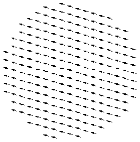
Induced flow fields for all state variables. From left to right: X, Y, Z, yaw, pitch, and roll.

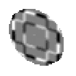
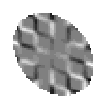
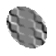
The six resulting Jacobian images. From left to right: X, Y, Z, yaw, pitch, and roll.

Bibliography

1

Y. Bar-Shalom and X. Li.
Estimation and Tracking: principles, techniques and software.
Yaakov Bar-Shalom (YBS), Storrs, CT, 1998.

2

J. R Bergen, P Anandan, Keith J Hanna, and Rajesh Hingorani.
Hierarchical model-based motion estimation.
In G Sandini, editor, Eur. Conf. on Computer Vision (ECCV). Springer-Verlag, 1992.

3

Frank Dellaert, Chuck Thorpe, and Sebastian Thrun.
Super-resolved tracking of planar surface patches.
In IEEE/RSJ Intl. Conf. on Intelligent Robots and Systems (IROS), 1998.

4

Frank Dellaert, Sebastian Thrun, and Chuck Thorpe.
Jacobian images of super-resolved texture maps for model-based motion estimation and tracking.
In IEEE Workshop on Applications of Computer Vision (WACV), 1998.

5

G. Hager and P. Belhumeur.
Efficient regions tracking with parametric models of geometry and illumination.
IEEE Trans. on Pattern Analysis and Machine Intelligence, October 1998.

6

G.D. Hager and P.N. Belhumeur.
Real time tracking of image regions with changes in geometry and illumination.
In IEEE Conf. on Computer Vision and Pattern Recognition (CVPR), pages 403-410, 1996.

7

T. Kanade, R. Collins, A. Lipton, P. Burt, and L. Wixson.
Advances in cooperative multi-sensor video surveillance.
In DARPA Image Understanding Workshop (IUW), pages 3-24, 1998.

8

R. Kumar, P. Anandan, M. Irani, J. Bergen, and K. Hanna.
Representation of scenes from collections of images.
In Representation of Visual Scenes, 1995.

9

A. Lipton, H. Fujiyosh, and R. Patil.
Moving target classification and tracking from real time video.
In IEEE Workshop on Applications of Computer Vision (WACV), pages 8-14, 1998.

10

S. J. Reeves.
Selection of observations in magnetic resonance spectroscopic imaging.
In Intl. Conf. on Image Processing (ICIP), 1995.

11

P. Rosin and T. Ellis.
Image difference threshold strategies and shadow detection.
In British Machine Vision Conference (BMVC), pages 347-356, 1995.

12

H.-Y. Shum and R. Szeliski.
Construction and refinement of panoramic mosaics with global and local alignment.
In Intl. Conf. on Computer Vision (ICCV), pages 953-958, Bombay, January 1998.

13

C. Stauffer and W.E.L. Grimson.
Adaptive background mixture models for real-time tracking.
In IEEE Conf. on Computer Vision and Pattern Recognition (CVPR), volume 2, pages 246-252, 1999.

About this document ...

Fast Image-Based Tracking
by Selective Pixel Integration

This document was generated using the LaTeX2HTML translator Version 98.1p1 release (March 2nd, 1998)

Copyright © 1993, 1994, 1995, 1996, 1997, Nikos Drakos, Computer Based Learning Unit, University of Leeds.

The command line arguments were:
latex2html -split 0 -show_section_numbers -local_icons -no_navigation framerate.tex.

The translation was initiated by on 1999-08-26