The QBD process that models a MAP/PH/1 queue length has a compact and convenient representation when we use the notation introduced above and in Section 2.2,
Consider a simpler case of an M/PH/1 queue, where
jobs arrive according to a Poisson process with rate ![]() , and
the service demand has a PH(
, and
the service demand has a PH(
![]() ) distribution.
The generator matrix for the queue length can be represented as
) distribution.
The generator matrix for the queue length can be represented as

Next, consider a MAP/M/1 queue, where
jobs arrive according to a MAP(![]() ,
,![]() ),
and the service demand has an exponential distribution with rate
),
and the service demand has an exponential distribution with rate ![]() .
The generator matrix for the queue length can be represented as
.
The generator matrix for the queue length can be represented as
Finally, consider a MAP/PH/1 queue, where
jobs arrive according to a MAP(![]() ,
,![]() ),
and the service demand has a PH(
),
and the service demand has a PH(
![]() ) distribution.
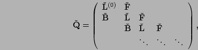
The generator matrix for the queue length can be represented as
) distribution.
The generator matrix for the queue length can be represented as
