Leveraging from the preceding analysis, we define our sampling-based
approach to profit prediction in general simultaneous, multi-unit
auctions for interacting goods. In this scenario, let there be ![]() simultaneous, multi-unit auctions for interacting goods
simultaneous, multi-unit auctions for interacting goods
![]() . The auctions might close at different times and
these times are not, in general, known in advance to the bidders.
When an auction closes, let us assume that the
. The auctions might close at different times and
these times are not, in general, known in advance to the bidders.
When an auction closes, let us assume that the ![]() units available are
distributed irrevocably to the
units available are
distributed irrevocably to the ![]() highest bidders, who each need to
pay the price bid by the
highest bidders, who each need to
pay the price bid by the ![]() th highest bidder. This scenario
corresponds to an
th highest bidder. This scenario
corresponds to an ![]() th price ascending auction.5 Note that the same bidder may place multiple
bids in an
auction, and thereby potentially win multiple units. We assume that
after the auction closes, the bidders will no longer have any
opportunity to acquire additional copies of the goods sold in that
auction (i.e., there is no aftermarket).
th price ascending auction.5 Note that the same bidder may place multiple
bids in an
auction, and thereby potentially win multiple units. We assume that
after the auction closes, the bidders will no longer have any
opportunity to acquire additional copies of the goods sold in that
auction (i.e., there is no aftermarket).
Our approach is based upon five assumptions. For
![]() , let
, let
![]() represent the
value derived by the agent if it owns
represent the
value derived by the agent if it owns ![]() units of the commodity
being sold in auction
units of the commodity
being sold in auction ![]() . Note that
. Note that ![]() is independent of the
costs of the commodities. Note further that this
representation allows for interacting goods of all kinds, including
complementarity and substitutability.6
The assumptions of our approach are as follows:
is independent of the
costs of the commodities. Note further that this
representation allows for interacting goods of all kinds, including
complementarity and substitutability.6
The assumptions of our approach are as follows:
By Assumption 3, the price predictor can generate predicted prices prior to considering one's bids. Thus, we can sample from these distributions to produce complete sets of closing prices of all goods.
For each good under consideration, we assume that it is the next one to close. If a different auction closes first, we can then revise our bids later (Assumption 4). Thus, we would like to bid exactly the good's expected marginal utility to us. That is, we bid the difference between the expected utilities attainable with and without the good. To compute these expectations, we simply average the utilities of having and not having the good under different price samples as in Equation 8. This strategy rests on Assumption 5 in that we assume that bidding the good's current expected marginal utility cannot adversely affect our future actions, for instance by impacting our future space of possible bids. Note that as time proceeds, the price distributions change in response to the observed price trajectories, thus causing the agent to continually revise its bids.
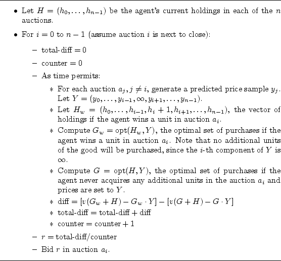
Table 1 shows pseudo-code for the entire algorithm. A fully detailed description of an instantiation of this approach is given in Section 5.
 |