Landmark Acquisition and Environment Identification
Abstract
Recognizing landmarks in sequences of images is a challenging problem for a number of reasons. First of all, the appearance of any given landmark varies substantially from one observation to the next. In addition to variations due to different aspects, an illumination change, external clutter, and changing geometry of the imaging devices are other factors affecting the variability of the observed landmarks. Finally, it is typically difficult to make use of accurate 3D information in landmark recognition applications. For those reasons, it is not possible to use many of the object recognition techniques based on strong geometric models.
The alternative is to use image-based techniques in which landmarks are represented by collections of images which capture the "typical" appearance of the object. The information most relevant to recognition is extracted from the collection of raw images and used as the model for recognition. This process is often referred to as "visual learning."
Models of landmarks are acquired from image sequences and later recognized for vehicle localization in urban environments. In the acquisition phase, a vehicle drives and collects images of an unknown area. The algorithm organizes these images into groups with similar image features. The feature distribution for each group describes a landmark. In the recognition phase, while navigating through the same general area, the vehicle collects new images. The algorithm classifies these images into one of the learned groups, thus recognizing a landmark.
Unlike computationally intensive model-based approaches that build models from known objects observed in isolation, our image-based approach automatically learns the most salient landmarks in complex environments. It delivers a robust performance under a wide range of lighting and imaging angle variations.
Table of Contents
2.2 Normalized Red Image and Features
3. Comparison between an image and an image
4. Grouping Images into Models and Comparison between an image and an model
4.3 Comparison between an Image and an Model
5.2 Perceptron or single layer network
5.3 Neural Network or Multi Layer Feed Forward Network
1. Introduction
Recognizing landmarks in sequences of images is a challenging problem for a number of reasons. First of all, the appearance of any given landmark varies substantially from one observation to the next. In addition to variations due to different aspects, illumination changes, external clutter, and changing geometry of the imaging devices are other factors affecting the variability of the observed landmarks. Finally, it is typically difficult to make use of accurate 3D information in landmark recognition applications. For those reasons, it is not possible to use many of the object recognition techniques based on strong geometric models.
The alternative is to use image-based techniques in which landmarks are represented by collections of images which capture the "typical" appearance of the object. The information most relevant to recognition is extracted from the collection of raw images and used as the model for recognition. This process is often referred to as "visual learning."
Unlike computational intensive model-based approaches that build models from known objects observed in isolation, our image-based approach automatically learns the most salient landmarks in complex environments. It delivers a robust performance under a wide range of lighting and imaging angle variations.
There are 2 steps in recognizing landmarks. In the training stage, the system is given a set of images in sequence. The aim of the training is to organize these images into groups based on similarity of feature distributions between the images. The size of the groups obtained may be defined by the user, or by the system itself. In the latter case, the system tries to find the most relevant groups, taking the global distributions of the images into account. In the second step, the system is given new images, which it tries to classify as one of the learned groups, or as belonging to the category of unrecognized images.
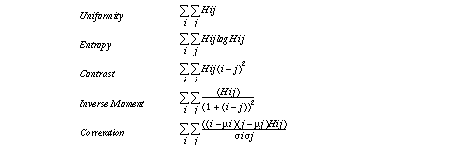
The basic representation is based on distributions of different feature characteristics. All these different kinds of histograms are computed for the whole image and for a set of sub-images. These features need to be invariant enough against variation of aspects, illumination, etc. Color and line segment-based features are used. A distance is defined to compare the distributions and to measure the similarity between images. This distance is then used to arrange the images in what are called groups. Each group is then characterized by a set of feature histograms. When new images are given to the matching algorithm, it evaluates a distance between these images and the groups. The system determines to which group this image is the closest, and a set of thresholds is used to decide if the image belongs to this group. The three methods evaluated in the matching algorithm, are the Mahalanobis distance or weighted euclid distance, the perceptron or single layer network, and the neural network or multi layer feed forward network.
Chapter 2 describes representing the image with the appropriate feature distributions. Chapter 3 shows a comparison between two images using the feature distributions. Because of the potentially wide variations in viewpoints, the images must be registered before comparing their feature distributions; an algorithm for fast, approximate image registration is described. Chapter 4 shows the grouping of images from a training sequence into groups to form landmark models, and presents a comparison between an image and a model. Chapter 5 describes the classification algorithm. Experimental data on training and test sequences from urban areas are presented throughout this paper.
2.1 Color and Edge Image
The object to be recognized is an outdoor scene. Its features vary widely due to different aspects and illumination. To avoid these effects, color image and edge image are used to compute some invariant features.
Color distribution can be a powerful attribute. However, color information must be used with caution because large regions may have little color information and the effect of shadows and illumination may change the color distribution drastically. The approach taken here is to consider only those pixels that have high enough saturation and to discard all the other pixels in the image. For the remaining highly saturated pixels, the normalized red value is used in order to minimize the effect of shadows and illumination.
The color values are resampled using a standard equalization. Specifically, the histogram of color values is divided into eight classes of roughly equal numbers of pixels. The color image is then coded on eight levels using those classes. This coarse quantization of color is necessary due to the potentially large color variations which make direct histogram comparison impossible. Line segments constitute the second class of features after linking and expansion of edge elements into segments. Several image attributes are computed using the image segments.
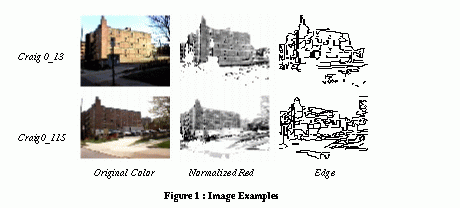
Figure 1 shows 2 images which have large differences in illumination but looks similar in the normalized red and edge image.
2.2 Normalized Red Image and Features
A pixel value of (i,j) in the original color image is described by rij, gij, bij, which correspond to red, green and blue. HSV values are computed as Hij , Sij , Vij , which correspond to hue, saturation and value. Red pixel Rij is computed as the following. Non-saturated or small value pixels do not have red value. Sky area is detected at the same time.
if ( Sij < Const || Vij < Const ) {
} else if ( sky condition 1 or 2 ) {
} else if ( rij == max(rij,gij,bij) ) {
Rij=rij*3/(rij+gij+bij) - 1 ; /* red value */
Sky condition 1 : rij > Const && gij > Const && bij > Const && (max(rij,gij,bij)-bij) < Const
Sky condition 2 : bij > Const && max(rij,gij,bij) == bij
Computed Rij is transformed into 0-255 scale, in which 0 designates the strongest red and 255 the weakest red. After making a histogram of Rij , it is divided into eight classes, each of which has a roughly equal number of. Rij , coded on eight levels using those classes. This normalized red image is very invariant against illumination or shadows.
We can use any color. In the case of this urban outdoor scene, trees are green, the sky is mostly blue, while the buildings, which occupy most of the scene, are red. For this reason, red is used as a color feature in our urban landmark recognition system.
The sky area is used in the first step of registration. Because it is difficult to extract feature points for registration due to unstable outdoor images, the sky area is used for approximate registration.
In this process, the original color image of 640x480 pixels is reduced to a 160x120 pixels red image. This reduction in size retains sufficient image quality and makes computational time shorter. Constant values are chosen empirically. Five kinds of texture values are computed in the normalized red image. Currently, entropy and contrast are implemented as features. Hij is the number of the pixel which itself has value i and next pixel has value j .
Cooccurence matrixes are computed from red normalized images. Since vertical and horizontal position operators are used, two kinds of matrixes and two kinds of the five texture values are computed.
2.3 Edge Image and Features
Edges are computed using Deriche's edge detector, and edge elements are linked and expanded into line segments. The input image is a 160x120 normalized red image. Five histogram features are computed from the edge image.
- Segment Length and Orientation : The histogram of the segment length is computed and normalized by the total number of segments. The histogram is taken over 20 buckets in the current implementation. Similarly, a histogram of the orientation of the segments is computed over 18 buckets.
- Intersecting Segments : Pairs of intersecting segments are identified and a histogram of their relative orientations is constructed over 18 buckets. The histogram is normalized by the total number of pairs.
- Parallel Segment Length and Orientation : Pairs of parallel segments are also identified and histograms of their lengths and orientations are computed. The histograms are normalized by the total number of parallel segments.
In implementation, only segment information whose start and end addresses are located in the active area is computed. This information is expanded to features after registration in matching. Note that these features can be computed only after registration.

3. Comparison between two images
Given a model image Im and an observed image Io , a distance can be computed by comparing attributes of the images. More precisely, Io is first registered with Im and the attributes are computed from the new, registered image. The global distance is defined as a sum of weighted local distances between attributes. In this section, registration and distance between two images are described. The distances are defined on only the top half part of the image, since the bottom typically contains more of the ground plane and little information of interest about the landmarks.
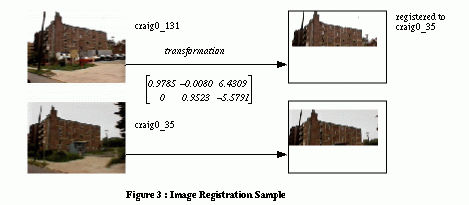
3.1 Registration
Given two images I1 and I2 , the registration problem consists of finding a transformation H such that H(I1) is as close as possible to I2 . This registration problem can be made tractable through a few domain assumptions. First of all, we are interested in landmarks that are far from the observer. Second, we assume that the images come from video sequences taken from a moving vehicle looking forward or from a transverse observer. As a result, the problem can be approximated by using an affine transformation H and by concentrating on the top half of the image, since the bottom typically contains more of the ground plane and little information of interest about the landmark.
Given those approximations, image registration is implemented in a two-step approach. In the first step, an initial estimate H0 is computed using only the data at the top of the image, which means sky area S(x) where x is the column number. A direct least-squares solution is used to minimize the sum of the squared differences taken over all columns.

The resulting parameters a and c correspond to the scale and translation along the rows of the image, and the translation along the columns, respectively. Those two parameters are by far the largest contributors to image change in typical video sequences taken from a moving vehicle.
The initial estimate of H is built by placing a and c in the first row of the matrix. H is then refined by comparing the images directly. In this refinement algorithm, the Sum of Squared Difference (SSD) between a fixed set of points of I1 and the corresponding set of points on I2 is computed using the current estimate of H . A change in the assignment of corresponding pixels that reduces the error is computed by moving pixels one by one. H is then estimated based on the updated correspondences. This algorithm reiterates until a stable value of H is reached This algorithm converges as long as the initial estimate H0 is close to the correct value. In particular, the algorithm performs well as long as large in-plane rotations do not contribute substantially to H . More general registration algorithms can be used in those situations.
The following shows the detail in the second detail registration process.
(X,Y) estimated address of (x,y) can be expressed by affine transformation H . We can add an additional constraint d=0 in order to avoid distortion by rotation.

Sampling pixels are every 10 by 10 points in the upper half image of I1 . These points are compared with corresponding points in Image I2. Given the address (x,y) , find i and j which minimize the difference between I1(x,y) and I2(x+i,y+j) . The difference means sum of difference in 5x5 pixels, the center of which is I2(x+i,y+j) . We can have some corresponding point pairs, both original points (x,y) and estimated points (X,Y) .

The pseudo-Inverse method is used to solve this equation, which minimizes SSD.
3.2 Local Distances
Local distance is computed for each attribute. There are four kinds of attributes: normalized red image, textures, edge image, segment histograms. Corresponding to these attributes are four kinds of local distances.
3.2.1 Local Distance in Normalized Red Image by Histogram
Sixteen sub-images are used from a regular 4x4 subdivision of the original image. The choice is a compromise between using a large number of small sub-images, thereby running risk of not having enough information in each sub-image, and using a small number of large sub-images, which may not have any advantage over using the entire image. The choice is also based on the average variation between images in the type of video sequences used in the test outdoor scenes.
Given two normalized red images, a histogram is computed in every sub-image. In comparing two histograms, the simplest method to express the difference is the sum of the squared difference between each element. However, registration cannot be precise enough to compare images directly by this method. The correction step is used to compensate for misregistration.
When the differences between the two histograms at element i and i+1 , dif(i) and dif(i+1) , are of opposite signs, their absolute values are decremented. This procedure is repeated over the entire histogram until no further adjustment is needed.
This procedure can be viewed as a coarse approximation of the earth-mover distance in which a cost is assigned in moving an entry from one histogram to another entry and the set of such motions for which cost is minimal is computed. By comparison, in the algorithm described above, zero cost is associated with a change of one entry in the histogram, and the final motion is determined using a sub-optimal algorithm. In practice, this approach effectively reduces the effect of misregistration.
while( further adjustment is needed ){
for( k=0; k<8; k++ ){ /* bucket number in histogram = 8 */
Dj(k) = H1j(k)-H2j(k) ; /* difference of histogram in subimage j */
After smoothing process, local distance is defined as the following.

Delta(j) shows whether the subimage k is used. In the current implementation, delta(j)=1 for top half subimages and delta(j)=0 for bottom half subimages. And the difference between histograms is defined as a kind of chi-square.
3.2.2 Local Distance in Red Texture
Comparing two images which have T1(i,j,k) and T2(i,j,k) , in which i=kinds of texture, j=direction vertical or horizontal and k=subimage, five kinds of local distance are computed corresponding to the five kinds of textures.

Delta(k) shows whether the sub-image k is used. In current implementation, delta(k)=1 for top half subimages and delta(j)=0 for bottom half subimages.
3.2.3 Local Distance in Edge Image
Line segments are extracted from edge images, and used to compare two images. Given two images, unmatched segments express the difference between them. Two segments are said to be matched if the following conditions are satisfied :
Local distance is defined as the sum of length of unmatched line segments.

3.2.4 Local Distance in Segment Histograms
Five kinds of local distances corresponding to five kinds of segment features are computed in almost the same way as the red image histogram.
3.3 Global Distance
The distances between individual attributes, which are called local distances, are combined into a single distance called global distance by using a weighted sum. This reflects the similarity of the images in appearance (color) and shape (edge distribution). When only 2 images are given, there is no rule to decide weight value. In this case, simply put weight 1. When sequence images are given, standard deviation can be used as a weight.

4. Grouping Images into Models and Comparison between an Image and a Model
The discussion above focused on comparing individual images. Because of the large variations in appearance, multiple images must be used for representing a given landmark. This means that groups of images that represent a single object of interest must be extracted from training sequences. In this section, we describe the algorithm which is used for extracting a small number of discriminating groups of images from a training sequence and tell how to use those groups as models for recognition.
4.1 Grouping
Let us denote the training sequence by Ii, i=1,2,...,n. The mutual distance between images in the sequence can be computed as dij=D(Ii,Ij) , where D is the global distance between image Ii and Ij defined above. In particular, it is implicit in this definition that Ii is registered to Ij as a part of the computation of D .
In computing global distance, the weight for each attribute is needed. From distance matrix dij , standard deviation is computed and used as a weight for each attribute.

Images for which the mutual distances are small are grouped into a number of clusters. Unlike general clustering problems in which the data can be arranged in clusters in an arbitrary manner, the training set has a sequential nature that can be used to make the grouping problem tractable. Specifically, images whose sequence numbers are far from each other cannot be grouped together because they were taken from locations distant from each other. Graphically, this means that we need only consider the values of dij for ij near the diagonal i=j . The exact meaning of "near" depends on the extent of the object of interest, the frequency at which images were digitized, and the rate of motion of the camera in the environment.
For a recognition system to be useful, only a small number of groups is relevant. More precisely, we are interested in the groups that have enough information, i.e., a large number of images with sufficient variation, and that are discriminating with respect to the other images. The second criterion is important because it is often the case that many groups look alike in a typical urban sequence. This is addressed by comparing the initial groups with one another and discarding those with high similarity to other groups.
In implementing this point of view, two conditions are added to grouping. An image which satisfies these conditions can be a landmark.
The first condition is to filter out images which are not appropriate for landmarks. Currently the following conditions should be satisfied in order for the image to be a landmark candidate :
- Sky Existence : The number of columns which have no sky or less than 10 sky pixels < Const
- Color Variation : The difference of analog intensity between 5th-1st red level > Const
- Segments Number : Total segment number < Const
The sky existence condition checks the existence of sky area. It is needed to approximate registration in the first step of registration. Color variation checks whether the image has a wide range in color. The low variation image has less information in color. An image which has many segments is confusing and not stable, e.g., most parts are trees, etc.
The second condition is the continuity or similarity in neighborhood images. This shows if image i has a continuity or similarity with image (i+1) . If this value is large, there is a large similarity gap between image i and image (i+1) , which means that image i and (i+1) cannot be in a same group. In the following equation, i'=i+1 and n=number of images in some range .

A pictorial representation of the set of values dij is shown in Figure 4 for the test sequence "craig3" and "5th98d." In this representation, the dij 's are displayed as a two-dimensional image in which the dark pixels correspond to large values. The diagonal, i.e., the values dii , is not shown since dii is always zero. Images which do not satisfy the former two conditions are now also shown. Images for which the mutual distances are small are grouped into a number of clusters.

Rejection of unreliable groups needs to be improved. Six candidates are automatically selected in this case, but 2 are rejected by hand because of similarity. Four models are used in the following recognition results.
4.2 Model Representation
Before being used for recognition, images which belong to a group must be collapsed into a model suitable for comparison with test images. There are two aspects to this. First, a reference image must be created as the core image representation of the model, usually the median image in the sequence, and all the other images are registered to it. Second, image attributes from all the images in the group must be collapsed into a single set of attributes.
The model is represented by two kinds of attributes, a red image with statistical information and line segments with probability. These representations are computed after registration to the core image.
4.2.1 Red Image with Statistical Information
In this model image, each pixel has a red value and a standard deviation value, computed as a mean and a standard deviation of group images.
4.2.2 Line Segments with Probability
Line segment information consists of start address and end address. In model representation, each segment has a probability. Probability is computed as the following. All segments in the core image are added to model segments and their probabilities are all 1. Segments in other images are matched to model segments nad probability is incremented if matched, and segment is added with probability 1 if unmatched. After all images are matched, probability is normalized by the number of images.
The matching algorithm is as same as the one used in computing local distance of edge image. Note that we cannot compute any feature values, for example histograms, because features can be computed only after registration in which the active area is fixed. The following shows edge and red images of four models.
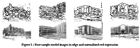
The lighter line segments correspond to probability, i.e., the darker line segments have a larger probability than the lighter ones.
4.3 Comparison between an Image and an Model
Run time recognition involves comparing a new image with all the models in order to determine the best match. The first step is to register an image to a model, and compute the attributes of the registered image over the overlapping region between an image and a model. The second step is to compute the global distance between an image and models. Local distance is discussed in this chapter, and global distance is discussed in the next chapter.
4.3.1 Local Distance in Normalized Red Image by Histogram
Local distance is computed in the same way as described in 3.2.1.
4.3.2 Local Distance in Red Texture
Local distance is computed in the same way as described in 3.2.2.
4.3.3 Local Distance in Edge Image
Line segments are matched in the same way as in comparing one image with another. Local distance is defined as the sum of the length of unmatched line segments by probability.

4.3.4 Local Distance in Segment Histograms
In computing a histogram of the model image, each element has not a number but a sum of probability of line segments which belong to the element. The comparison process is the same as in comparing one image with another. Note that the histogram has not integers, rather, it has real numbers.
5. Recognition
Given an image and some models, local distances dij(k) are computed, in which i=image serial number, j=model number, k=attribute number. The issue is how to compute the score or global distance Gij and how to decide which model the image belongs to. We present three kinds of methods : (1) Mahalanobis Distance (2) Perceptron or Single Layer Network (3) Neural Network or Multi Layer Network.
5.1 Mahalanobis Distance
Assume dij(k) is a set of local distances in the training sequence of model j . The variance-covariance matrix Cj and linear discriminant function can be computed from dij(k) .

dij(k) = local distance ; i=image number of training sequence, j=model number, k=attribute number
Cj = Variance-Covariance matrix
M1j = mean vector of group 1 images which belongs to model j
M2j = mean vector of group 2 images which doesn't belong to model
D = dij(k), Linear Discriminant Function :
We assume that variance-covariance matrixes are equal in group 1 and group 2. In a special case, we can put zero value for Cj except the diagonals. This distance can be said to be weighted euclid distance.
5.2 Perceptron or Single Layer Network
The linear discriminant function can be learned by the perceptron learning algorithm. In our case, a pattern vector d corresponds to dij(k) . For a while , we omit subscript j which shows the model number. A pattern vector appears as a point in the pattern space, and this space can be partitioned into two parts by a linear discriminant function described as f( w , d )= w t d where d =( d1,d2,...,dn,1 ) t , w =( w1,w2,...,wn,wn+1 ). w represents weight vectors.
The (n+1) th dimension is added as a constant. The classification criterion is as follows :
if f( w , d )>0 then d belongs to group 1, else belongs to group 2
The problem is to find a solution of w which satisfies this condition. If all d 2 which belong to group2 are replaced by their negatives, - d 2 , the solution region of w should satisfy f( w , d )>0 for all d . We can add a parameter b as a margin and the equation is f ( w , d )> b.
Weight vector w is obtained by using gradient techniques. The (k+1) th weight vector can be obtained by adding some multiple of misclassified samples to the k th weight vector.

There are two issues. One is that the classifier f should be located as near to the center between 2 groups as possible. Another is that irregular date has a significant effect on the classifier ; this should be avoided as much as possible.
Learning is controlled by margin value. In learning, misrecognition means f ( w , d )< M where M is margin value. By increasing the margin value in every learning step, the classifier can be located near the center.
When group 1 contains concept landmark images and group 2 does not contain concept images, misclassification from group 1 to group 2 means that the system cannot recognize the landmark ; this means not misrecognition, but rather rejection. But misclassification from group 2 to group 1 means that not-concept image is recognized as a concept, which is misrecognition. We can say the former misclassification can be allowed comparing to the later one. In the learning stage when margin value is increased, misclassification images from group 1 to group 2 are excluded from learning data in order to avoid the problem of irregular data.
for( M=0; M<1.0 ; M=M+0.01 ){ /* M = margin value */
Exclude misclassified data and include classified data in group 1 ;
In the perceptron learning stage, learning stops when learning converges or the learning loop count exceeds the limit, currently 5000. Margin value is increased from 0 to 1.0 in 0.01 increments. The sum of weights is normalized to be 1.
Classifiers are computed corresponding to margins and each classifier has a score computed as the following.

MisClassification1 = that of group 1 to group 2, MisClassification2 = that of group 2 to group 2, Excluded-Data- Number = that of group 1. Parameter p1, p2, p3 means that there is a penalty value for each. The classifier which has the minimum score is the best one.
5.3 Neural Network or Multi Layer Feed Forward Network
The learning algorithm is almost the same as that for perceptron learning with margin control. It has the following features.
- The model is 2 layer feed forward network.
- In the hidden units, the last one is constant unit.
- The learning algorithm is back propagation with general delta rule.
- The learning process is controlled by margin control algorithm described above.
- The weights are control by the following equation, in which the weight values are replaced after every process of back propagation.

The score is computed in every margin step, and the best classifier, which has the minimum score, is selected.
6. Experimental Results
Four kinds of data sequences and four kinds of classifiers were evaluated. The classifiers included weighted euclid distance, perceptron, neural network with 4 hidden units and neural network with 6 hidden units. Images of concept had a large variation of illumination and camera angle, due to the fact that they were taken at about 10 different times, which means during sunshine or cloudy weather, morning or evening, etc.
Data Sequence 1 : Recog Learning
---> Learning Sequence for Recognition = Images which belong to the concept
---> Test Sequence for Recognition = Image which belongs to the concept, except for data sequence 1
Data Sequence 3 : Reject Learning
---> Learning Sequence for Rejection = Images which don't belong to the concept
---> Test Sequence for Rejection = Images which don't belong to the concept, except for data sequence 3
In Table 1, even number learning, the learning sequence is selected as even numbered images in whole sequence. Both sequences have almost same images. In Table 2, random selected 30% data learning, 30% images are selected at random. In table 3, 50% images are selected at random.
The value in the tables are recognition rate. In recog learning/test, this rate means correctly recognized, and 100-rate means rejected. In reject learning/test, this rate means misrecognized, and 100-rate means correctly rejected.
In weighted euclid distance, the logic to match sky area is added to avoid misrecognition. Strictly speaking, matching sky is not pattern recognition but form recognition. This distance is shown only for purposes of comparison with the others.
The misrecognition rate can be decreased by adding this logic to the others, but the recognition rate will correspondingly decrease. Strictly speaking, sky matching cannot be said to be recognition, because it compares only the form of the detected sky area. We can say the following based on the results:
Perceptron has a stable recognition rate of about 85% in learning and test images
The neural network has almost 100% recognition rate in learning, but about 80 to 90% in test images.
Figure 6 shows some example images recognized in even data learning.
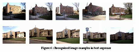
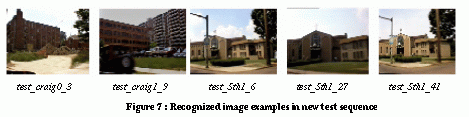
Additional images were taken and used for experimental results. Strictly speaking, images in Figure 6 were almost all taken in autumn and winter, while images in Figure 7 were taken in summer. So illumination and color, especially shades of green, differs drastically.
Weighted Euclid Distance |
||
Perceptron |
||
Neural Network(Hidden 4) |
||
Neural Network(Hidden 6) |
||
Recognized image samples are shown in Figure 7.
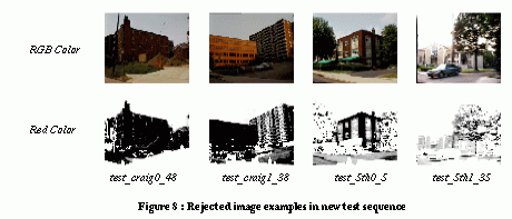
The results show that the algorithm can recognize effectively under huge variation in conditions. However, the images in Figure 8 are excluded from the results because of too much variation. The first and second have little variation in color because of illumination. In the third one, the landmark building is occluded by trees. In the fourth one, the landmark building is occluded by color and the color is not saturated.
7. Conclusion
Results on image sequences in real environments show that visual learning techniques can be used for building image-based models suitable for recognition of landmarks in complex scenes. The approach performs well, even in the presence of significant photometric and geometric variations.
Several limitations of the approach need to be addressed. First of all, rejection of unreliable groups needs to be improved. It is often the case that some groups look alike in a typical urban sequence. Those with high similarity to the other groups should be discarded automatically.
Second, images that do not contribute information should be filtered out of the training sequences. Currently the image need to satisfy some conditions to be a landmark candidate. However they are not sufficient enough.
Third is an integration of algorithm to vehicle system and demonstration. In order to execute the real time recognition, it is essential to optimize the time performance.
References
Bach et al. The Virage Image Search Engine:An Open Framework for Image Management. SPIE Proc. Image Storage and Retrieval. 1996.
S. Carlsson. Combinatorial Geometry for Shape Indexing. Proc. Workshop on Object Representation for Comp.Vision. Cambridge. 1996.
F. Cozman. Position Estimation from Outdoor visual landmarks. Proc. WACV'96. 1996.
P. Gros, O. Bournez and E. Boyer. Using Local Planar Geometric Invariants to Match and Model Images of Line Segments. To appear in Int. J. of Comp. Vision and Image Underst.
R. Horaud, T. Skordas and F. Veillon. Finding Geometric and Relational Structures in An Image. Proc. of the 1st ECCV. Antibes, France pages 374-384, April 1990
B.Lamiroy and P. Gros. Rapid Object Indexing and Recognition Using Enhanced Geometric Hashing. Proc. of the 5th ECCV, Cambridge, England, pages 59-70, vol. 1, April 1996.
R.W. Picard. A Society of Models for Video and Image Libraries. IBM Systems Journal, 35(3-4):292-312. 1996.
D.A. Pomerleau. Neural network-based vision processing for autonomous robot guidance. Proc. Appl. of Neural Networks II. 1991.
Y. Rubner, L. Guibas, C. Tomasi. The Earth Mover's Distance, Multi-Dimensional Scaling, and Color-Based Image Retrieval. Proc. IU Workshop. 1997.
C. Schmid and R. Mohr. Combining Greyvalue Invariants with Local Constraints for Object Recognition. Proc. CVPR. San Francisco, California, USA. pages 872-877, June 1996.
M.J. Swain, D.H. Ballard. Color Indexing. Int. J. of Comp.Vision, 7(1):11-32.1991.