Homework 2
Juan Fasola
ID: jfasola
1. Below is a screen shot of the program running. It displays
the start location (in red), the robot (in blue) at the goal location,
and the
path taken by the Bug1 algorithm (in orange). The workspace obstacles
are in black and were loaded from an input PGM file.

I used OpenGL to draw the graphics for the program, and it is written
in C. The program takes one command line argument that is the
background image, or rather, the workspace file. The file must be a PGM
image file, with the free space represented by white pixels (255) and
obstacles in black (0). It also must be 400x300, the same size as the
program window. Loading a workspace file makes creating wacky obstacles
very easy (just need to draw them using a paint program). Example
program call: ./hw2 workspace.pgm
Implementation Details:I chose to implement the Bug1 algorithm.
The algorithm starts out by loading in the workspace file from the
specified PGM file from the command line and then creating the
configuration space by expanding the obstacles by the robot radius and
some buffer zone (so that the robot doesn't actually touch the
obstacles), both parameters are easily tunable within the code. For the
movie examples, I used a robot radius of 7px and buffer zone of 1px.
Once the configuration space is created the workspace is displayed on
the screen.
Now the user can select the starting point and goal point by
simply clicking on desired positions within the image window. The
starting point is displayed in red and the goal point in green. To
change the points at any time, just click somewhere else and the points
are updated. Once both points are chosen, the user can start the Bug1 algorithm by hitting the 'Enter' key.
The Bug1 algorithm will travel directly from the start towards the
goal, if a configuration space obstacle is hit, the robot
circumnavigates around the entire obstacle while keeping track of the
point along the obstacle that is closest to the goal. Once the robot
returns to the initial hit point, it moves back to the closest point to
goal by taking the shortest route along the obstacle boundary. Once the
robot reaches this point, it moves towards the goal again, if it
immediately runs into the obstacle it had just followed around, the
algorithm returns in FAILURE. If at any point during the algorithm the
robot position is at the goal, the algorithm returns in SUCCESS.
If the algorithm terminates succesfully, the path taken is
displayed in orange. If it fails to find a solution, the robot turns
red in color and no path is shown. After the algorithm completes, and
really at any time, two new start and goal points can be chosen by
clicking on the program window, without having to restart the program.
Figures: Below are examples of what the configuration space
looks like for two different workspaces, generated by the program for
use in the Bug1 algorithm, by expanding the obstacles an amount equal
to the robot radius + some buffer zone (1 px).

Robot radius = 7 px
|
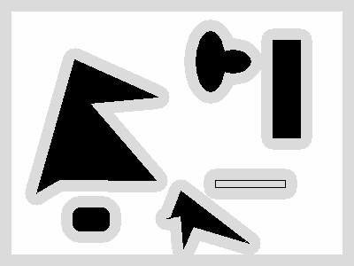
Robot radius = 12 px
|
2. Movies
3. I chose the Bug1 algorithm because it's a good starting
point for the Bug2 algorithm, unfortunately I ran out of time before
the due time to create the Bug2 algorithm and test it appropriately. I
had originally planned to make both algorithms, but the Bug1 algorithm
is still cool anyways by itself.