Big-O#

Overview#

We can measure the run time, spatial complexity, or general resource consumption of a given function through Big-O notation. Informally, if the function my_fn(x) runs in \(O(f(n))\), this means that when the input x is of size \(n\), the worst-case scenario run time of my_fn(x) is asymptotically a constant multiple of \(f(n)\).

In this class, \(n\) could be the number of data points, the length of the input sequence, or the number of nodes in a tree, for example.

Note that run time here refers to the number of algorithmic steps that the function takes rather than wall-clock time.

Definition and Mathematical Properties#

For the purposes of this course, (and most future MLD courses you may or may not take), it’s best to think of big-O for comparing two arbitrary functions, which we will call \(f\) and \(g\) respectively. For simplicity, we’ll assume that both \(f\) and \(g\) are defined over \(\mathbb{R}_+\) (that is, \(f\) and \(g\) only take positive real numbers as inputs), which is enough for this course. Formally, Big-O is defined as:

Definition 1: Big-O Definition#

If \(f(n) \in O(g(n))\), then there exists some \(c, n_0 \in \mathbb{R}_+\) such that:

\[\forall n \ge n_0, \quad f(n) \le c g(n)\]

(Note: if you’ve seen Big-O before, you may be more familiar with the notation \(f(n) = O(g(n))\). We avoid using this alternative as the equality operator implies a certain degree of symmetry that is not present.)

In words, this means that if \(f(n) \in O(g(n))\), then at some point as the inputs increase, \(f(n)\) will always be less than or equal to a constant multiple of \(g(n)\). Usually, \(f\) is the function whose runtime we are measuring. It is our job to find a function \(g\) that asymptotically upper bounds \(f\).

An Aside on Verbiage#

It can sometimes be confusing to talk about big-O in the context of computer science and the math behind it, as functions like \(n!\) are simultaneously described as “fast-growing” and “slow.” This is not incorrect: calling \(n!\) “fast-growing” refers to the fact that as \(n\) increases, \(n!\) quickly explodes (1, 1, 2, 6, 24, 120, 720, 5040, …), while calling \(n!\) “slow” refers to the fact that an algorithm that runs in \(O(n!)\) time takes a constant multiple of \(n!\) steps to run, which can take a long time! Normally, “fast-growing” is used more when talking about big-O in the pure mathematical sense (e.g., comparing arbitrary functions), while “slow” is used more in computer science when talking about run-time complexity, so we expect you to be comfortable with both!

Standard Complexity Classes#

While the big-O bound for any function \(f\) can be defined by any other valid function \(g\), in computer science we generally only talk about the following complexity classes (shown in increasing order of complexity):

\(O(1)\): Constant time – While the input size increases, the function’s runtime is unaffected.
\(O(\log(n))\): Logarithmic time
\(O(n)\): Linear time
\(O(n\log(n))\): Log-linear time
\(O(n^2)\): Quadratic time
\(O(n^p)\): Polynomial time, for some \(p > 2\)
\(O(p^n)\): Exponential time
\(O(n!)\): Factorial time

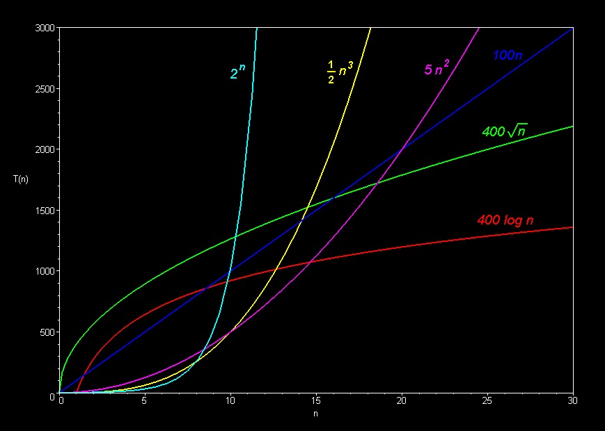
Here is a visualization of a few of these classes:

Big-O Complexity Classes

Big-O Scales

Source: here

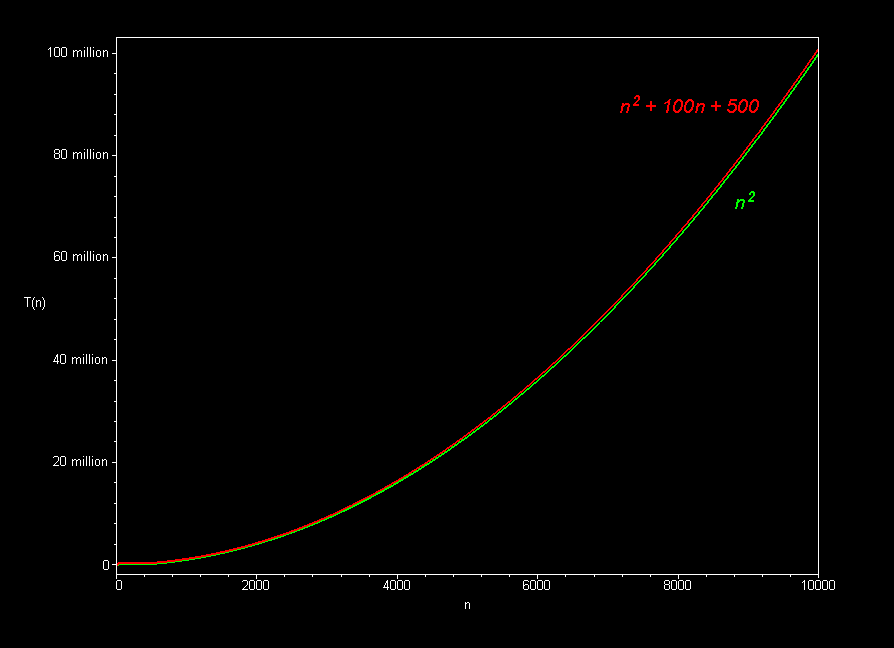
The second image plots two functions with the same leading coefficient, but one has added terms of a lower order. The second function is asymptotically equivalent to the first, but the added terms make it grow faster for small values of \(n\). This is why we only care about the leading term when determining Big-O complexity.

Big-O Properties#

Based on this definition, we get a few interesting properties as a consequence:

Definition 2: Transitivity Property#

For three functions \(f, g, h\) all on \(\mathbb{R}_+\), if \(f(n) \in O(g(n))\) and \(g(n) \in O(h(n))\), then \(f(n) \in O(h(n))\).

A result of the transitivity property is that a function \(f\) does not have a unique big-O bound, as we can always come up with faster-growing functions than \(f\). However, in computer science we normally want the tightest Big-O bound in order to formalize what realistically happens “in the worst case.”

Definition 3: Law of Addition#

If \(f(n) = f_1(n) + f_2(n)\) for some functions \(f_1, f_2\) such that \(f_2(n) \in O(f_1(n))\), then \(f(n) \in O(f_1(n))\).

In words, this means that we only care about the fastest growing part of a function to determine its Big-O complexity. So if \(f(n) = 5n^3 + 2n\), then \(f(n) \in O(n^3)\) (i.e., we can disregard the \(2n\) term, as asymptotically \(5n^3\) becomes much larger than \(2n\)).

Definition 4: Logarithmic Equivalence (Change of Base Rule for Logarithms)#

If \(f(n) = \log_p(n)\) and \(g(n) = \log_q(n)\) for two bases \(p, q \in \mathbb{N}\), then \(f(n) \in O(g(n))\) and \(g(n) \in O(f(n))\).

To show that this is true, recall the log rule that \(\log_a(b) = \frac{\log(b)}{\log(a)}\) where \(\log\) is the natural log. Given this, \(f(n) = \frac{1}{\log(p)}\log(n)\) and \(g(n) = \frac{1}{\log(q)}\log(n)\), and thus \(f(n)\) and \(g(n)\) are equivalent up to a constant. This formula holds in general for any log base, not just natural logs.

Code Examples#

Linear Search#

for i in range(n):
    if data[i] == target:
        return i
return -1

In the worst-case scenario, LinearSearch performs a constant-time operation \(n\) times. As such, we say the runtime of LinearSearch is in \(O(n)\).

Binary Search#

left = 0
right = n
while left < right:
    middle = (left + right) // 2
    if data[middle] < target:
        left = middle + 1
    else:
        right = middle

In each iteration until \(left \geq right\), BinarySearch performs constant-time operations. This means we can determine the asymptotic runtime of BinarySearch by the number of iterations until the function returns. In this case, that is \(\log_2(n)\), which is the maximum number of times you can divide a sequence of \(n\) numbers in half. As such, BinarySearch is in \(O(\log n)\).

Forward-Backward Algorithm#

alpha[0]['<START>'] = 1
for t in range(1, T):
    for s_j in states:
        alpha[t][s_j] = A[j, x_t] * sum(B[k, j] * alpha[t-1][s_k] for s_k in states)

This is the forward-backward algorithm. Do not worry about what the function does for now. Instead, focus on the runtime analysis. We multiply the number of iterations of all three loops: the outer loop (\(T\) iterations), the inner loop (\(J\) iterations), and the implicit loop in the summation (\(J\) iterations). As such, ForwardBackward is in \(O(J^2 T)\).

Big-O

Contents