Optimal Cone Singularities for Conformal Flattening
SIGGRAPH 2018 / ACM Transactions on Graphics 2018

Angle-preserving or conformal surface parameterization has proven to be a powerful tool across applications ranging from geometry processing, to digital manufacturing, to machine learning, yet conformal maps can still suffer from severe area distortion. Cone singularities provide a way to mitigate this distortion, but finding the best configuration of cones is notoriously difficult. This paper develops a strategy that is globally optimal in the sense that it minimizes total area distortion among all possible cone configurations (number, placement, and size) that have no more than a fixed total cone angle. A key insight is that, for the purpose of optimization, one should not work directly with curvature measures (which naturally represent cone configurations), but can instead apply Fenchel-Rockafellar duality to obtain a formulation involving only ordinary functions. The result is a convex optimization problem, which can be solved via a sequence of sparse linear systems easily built from the usual cotangent Laplacian. The method supports user-defined notions of importance, constraints on cone angles (e.g., positive, or within a given range), and sophisticated boundary conditions (e.g., convex, or polygonal). We compare our approach to previous techniques on a variety of challenging models, often achieving dramatically lower distortion, and demonstrating that global optimality leads to extreme robustness in the presence of noise or poor discretization.

PDF, 15MB
@article{Soliman:2018:OCS,
author = {Soliman, Yousuf and Slep\v{c}ev, Dejan and Crane, Keenan},
title = {Optimal Cone Singularities for Conformal Flattening},
journal = {ACM Trans. Graph.},
volume = {37},
number = {4},
year = {2018},
publisher = {ACM},
address = {New York, NY, USA},
}
Presentation
Thanks to Henrik Schumacher for useful references to algorithms from optimal control, to Rohan Sawhney for implementation help with BFF, and to Alex Huth for sharing cortical surface data. This work was sponsored in part by NSF Awards CCF 1717320 and DMS 1516677, a CMU Summer Undergraduate Research Fellowship (SURF), and gifts from Autodesk Research and Adobe Research.
This material is based upon work supported by the National Science Foundation. Any opinions, findings, and conclusions or recommendations expressed in this material are those of the author(s) and do not necessarily reflect the views of the National Science Foundation.
|
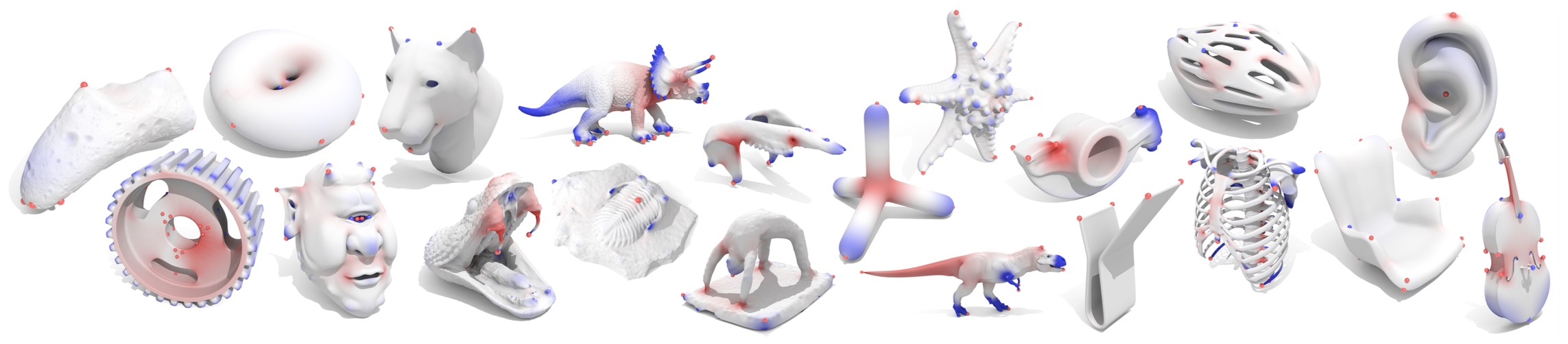
Example meshes from the paper with optimal cone singularities, and associated conformal flattenings.
 optimal-cones-data.zip Wavefront OBJ, 25MB
|
Supplemental
Conformal Cone Parameterization Through Optimal Control — Yousuf Soliman's MS thesis; contains additional background and details. (88MB)
Figures

A conformal cone parameterization is equivalent to flattening a smooth surface, like the sphere, over a polyhedron, which can then be cut and unfolded into the plane without further distortion. By adding more and more cone points, one can make area distortion arbitrarily small.

Intuitively, it might seem that the best place to put cones is in regions of high curvature K or large scale distortion u. However, the optimal location may actually be a point that is nearly flat---helping to explain the suboptimal behavior of greedy algorithms. Here we place either one cone (top) or eight cones (bottom); notice that even for a larger number of cones, the optimal configuration continues to include cones in flat regions.

Even with fewer cones and much smaller total cone angle, our cone placement strategy (MAD) yields far lower area distortion than previous methods. This effect is especially apparent on shapes like the brain, which do not have obvious peaks of curvature.
Left: cones placed according to standard L2 energy. Right: cones placed by re-weighting the L2 energy (and regularizer) according to local feature size. Both cone configurations are globally optimal solutions to different problems.
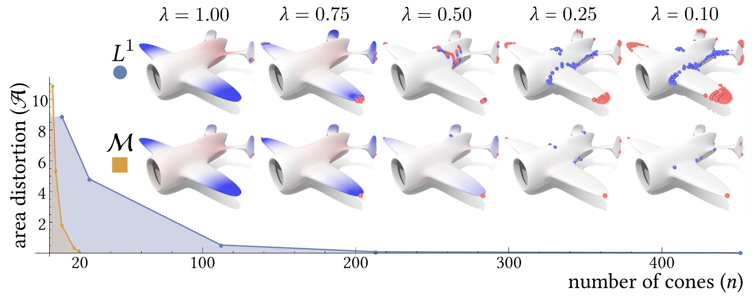
Using L1 regularization yields unpredictable results that are not concentrated on isolated points (top row), whereas using the measure norm yields well-behaved solutions that properly represent cone singularities (bottom row). Tuning the parameter λ does not improve the L1 result; moreover, the measure-based approach achieves smaller area distortion using dramatically fewer cones (as shown in the plot at bottom).

Different treatments of boundary data allow us to minimize L1 area distortion with (a) no cones, (b) optimal cones and isometric boundary conditions, (c) optimal cones and optimal boundary conditions; we can also find the least-distorting maps with (d) polygonal and (e) convex boundaries.
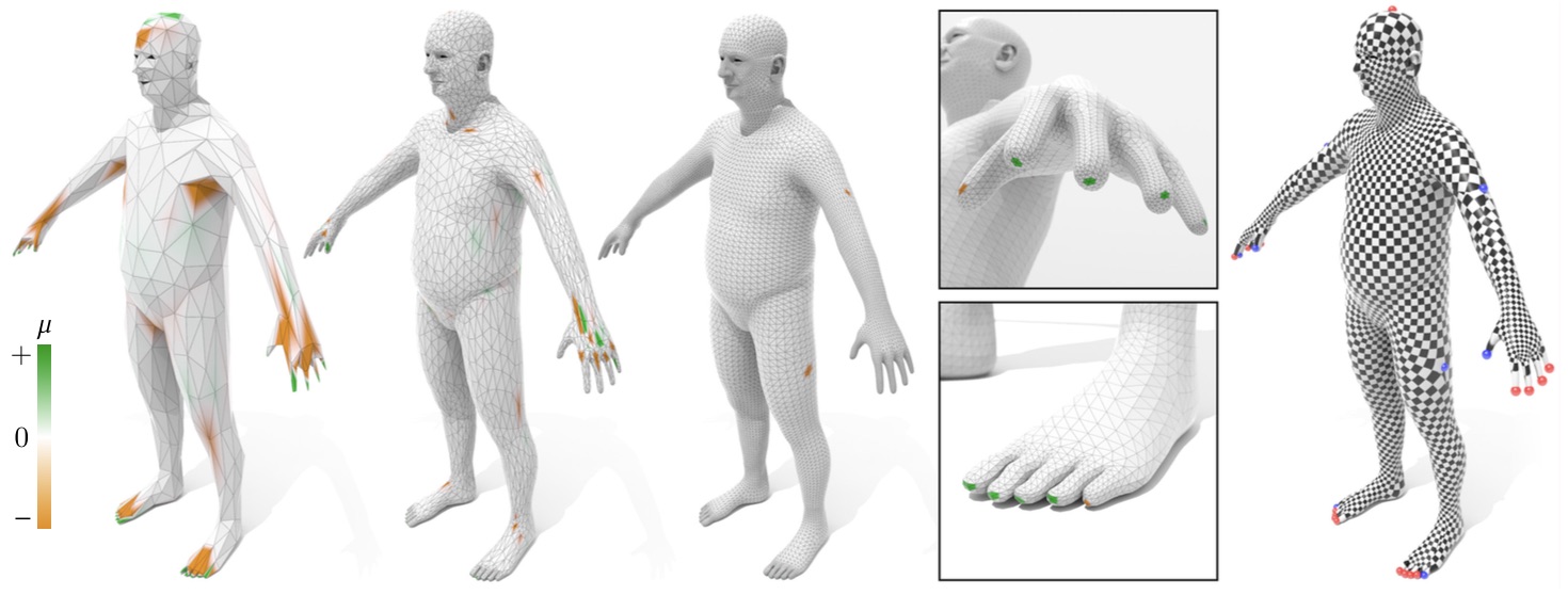
Mesh hierarchy built on the Old Man Multires model; here we use only three levels. Compared to solving directly on the full-resolution 30k triangle mesh, we obtain a speedup factor of about 23x (from 14.77s to about 0.62s). Colors indicate the optimal regularized measure; in the final (fine) mesh the measure is exactly concentrated onto isolated vertices. Far right: The resulting parameterization has only 32 cones, with a total angle of 18.86π.
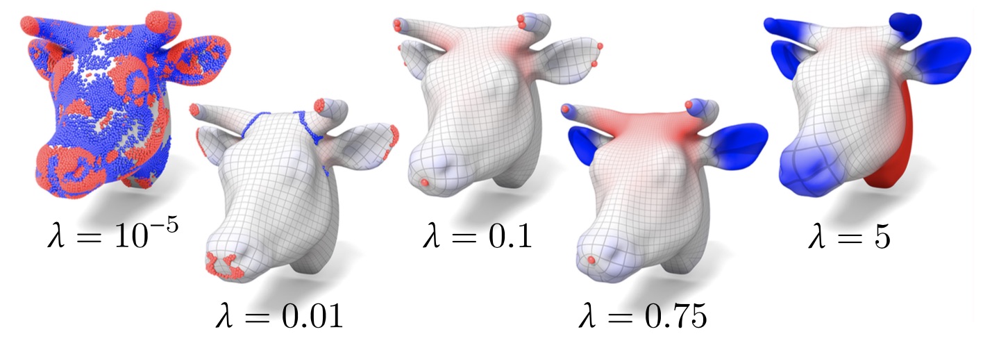
The parameter λ controls the strength of the penalty on the total cone angle, and in turn, influences the number of cones. For values above 1 (strong penalty) we tend to see that no cones are placed. For values very close to zero (weak penalty) the curvature measure stops being sparse, and we get cones with small angles placed densely across regions or along curves rather than at isolated points.

The parameter λ has a very consistent behavior across different surfaces, typically producing a similar density of cones.
Using a default parameter λ = 1/2 allows one to flatten a wide variety of different models without any explicit tuning or adjustment.

Finding just the right configuration of cones and angles can sometimes dramatically reduce area distortion. Here, MAD almost completely eliminates area distortion using just 8 cones (far right). Using the same number of cones in CPMS (far left) yields far greater distortion; alternatively, one can drive the distortion to similar levels (center left) but using far more cones. GPIF yields higher distortion than MAD, even after placing a whole ring of cones around the top of the head.

Optimal singularities for direction fields (top) are not necessarily good for conformal flattening (bottom).

Our method produces consistent results on meshes of very different resolution (top row) and is also robust to meshing artifacts such as noise (bottom left), anisotropy (bottom center), and severely non-Delaunay elements (bottom right). The same λ value is used in all examples.

Variable density mesh. Left: CPMS places far more singularities in finely tessellated regions, where Green's functions are better resolved; note that many spheres overlap due to close clustering of cones. Center: GPIF also violates symmetry, and achieves lower distortion than MAD only by using about twice as many cones. Right: MAD achieves low area distortion using a symmetric arrangement of just a few cones, and with small total cone angle.

Stress test of robustness. Methods that place cones according to peaks in scale factors (left) or based on curvature (center) may be confounded by outliers; here we consider an extreme case where near-invisible spikes are added to a mesh, leading to cone configurations that are impossible to parameterize (bottom). Since our method minimizes an integral energy, it is generally not confounded by outliers or noise, in this case ignoring the spikes and leading to a high-quality parameterization (right).

We can selectively restrict cone placement to any user-specified region. Here for instance, by shooting rays (top left) we can determine the region visible from a particular point of view (bottom left). If we now restrict our search to this region---while still penalizing distortion in the front---singularities that would ordinarily appear on the front (center) instead get “pushed” to the back (right).

Left: When finally mapped to the plane a cone flattening of a surface (such as this brain) may have local noninjectivity at negative cones, unless these cones are cut into sufficiently small pieces (see zoom). Right: finding an optimal solution with only positive cones avoids this source of local noninjectivity.

Left: in the absence of any bounds on cone angles, an optimal configuration for this model is to place eight equal cones corresponding to an octahedron. Center: if we now limit angles to the range [0,π], we get a configuration that has eight cones of π/2, but not at the corners of a cube as one might expect: instead, we get a flattening to a cuboid with unequal lengths. Right: the more intuitive configuration with cones at cube corners yields higher area distortion.
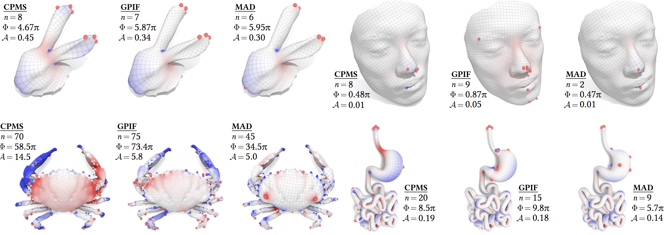
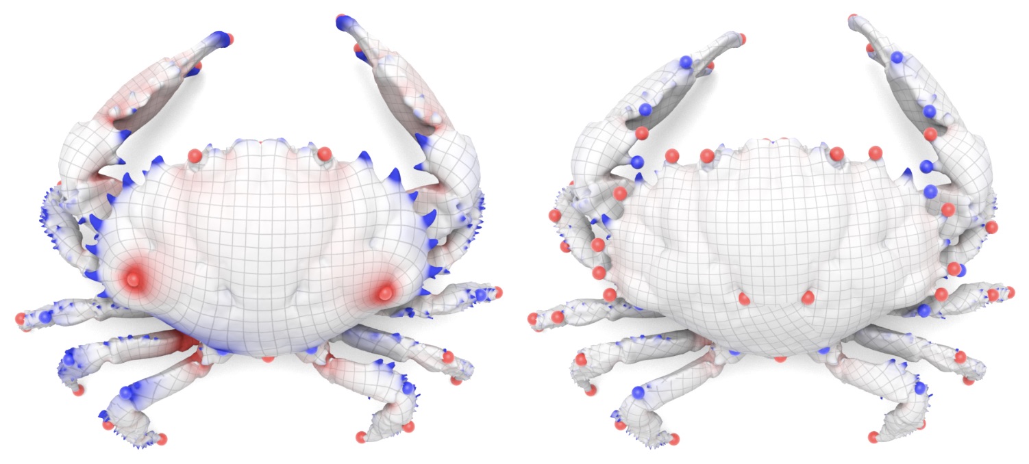
More comparisons. On models with simple geometry (top row) greedy or region-growing strategies can work quite well, though MAD still performs slightly better. On more challenging models such as the crab (bottom left) the gap typically widens---note also the high degree of symmetry for MAD.