Large language models (LLMs) have led to significant progress in various NLP tasks, with long-context models becoming more prominent for processing larger inputs. However, the growing size of the key-value (KV) cache required by Transformer architectures increases memory demands, especially during the decoding phase, resulting in a significant bottleneck. To address the memory bottleneck, sparse attention methods approximate full attention using only a small set of critical tokens. Current sparse attention mechanisms designed to alleviate this bottleneck have two main drawbacks: (1) they often struggle to identify the most relevant tokens for attention accurately, and (2) they fail to account for the spatial consistency of token selection across successive Transformer layers, which can result in reduced performance and increased overhead in token selection.

TL; DR

• This blog introduces TidalDecode , a streamlined and efficient algorithm and system for fast and high-quality LLM decoding, utilizing position persistent sparse attention .
• To address KV cache distribution shifts, TidalDecode further introduces a cache-correction mechanism that periodically refills the KV cache using full attention for sparsely decoded tokens.
• Empirical evaluations demonstrate the effectiveness and efficiency of TidalDecode, showing that TidalDecode significantly outperforms existing sparse attention methods and achieves up to 2.1x decoding speedup ratio compared with the state-of-the-art attention serving framework.

Background

Large Language Model Serving

LLM inference involves two separate stages: prefilling and decoding. The prefilling stage computes the activations for all input tokens and stores the keys and values for all tokens in the key-value (KV) cache, allowing the LLM to reuse these keys and values to compute attention for future tokens. The LLM decodes one new token in each decoding stage using all input and previously generated tokens. The KV cache size grows linearly in the sequence length. For instance, with a context length of 128K tokens, the KV cache of LLama2-7B with half-precision can easily reach 64GB,

num_layers × num_kv_head × head_dim × seqlen × sizeof(fp16) × 2 (for K+V) =
32 × 32 × 128 × 128K × 2 bytes × 2 = 64GB.

creating substantial memory pressure for LLM serving. In addition, the LLM decoding stage is memory-bounded since decoding one new token requires accessing all previous tokens in the KV cache, making KV cache access the primary bottleneck for long-context LLM decoding. This memory-bound nature severely limits the scalability and efficiency of LLM serving.

Sparse Attention

To address this problem, recent work has introduced sparse attention, which approximates full attention using a small portion of tokens with the highest attention scores. Compared to full attention, sparse attention reduces computation cost and memory access while preserving the LLM’s generative performance ( Ge et al., 2024 ; Zhang et al., 2023 ). Existing sparse attention techniques can be classified into two categories: eviction - and selection -based methods.

Eviction-based sparse attention

StreamingLLM ; H2O propose to reduce KV cache memory usage by evicting tokens that are considered less relevant during inference. These suffer from potential performance degradation, especially in tasks where every token may carry crucial information (e.g., Needle-In-The-Haystack tasks), since tokens with high importance for a future decoding step can be mistakenly evicted as the generation proceeds, which makes selection-based methods more popular choices in the latest sparse attention works.

Selection-based sparse attention

Instead of evicting past tokens in the KV cache, Child et al. (2019) , Reformer , Performer , Quest , SparQ , MagicPIG preserve the full KV cache and only select important tokens to attend with the attention module on the fly.

More specifically, Child et al. (2019) leverages a fixed attention mask to select tokens while Reformer , Performer , Quest , SparQ and MagicPIG aim to identify and retain the most relevant tokens at each layer by approximating attention scores with pruned query/key vectors or locality-sensitive-hashing.

Although these methods are more selective, they operate independently at each layer and are not guaranteed to obtain the ground-truth tokens with the highest attention scores, failing to capture token relevance patterns that persist across layers. Moreover, attention score estimation algorithms can introduce unnecessary complexity, diminishing the practical efficiency gains they are designed to achieve.

Improving upon prior works, TidalDecode leverages a shared pattern of the most important tokens across consecutive layers to further reduce the computational overhead and memory access required for token selection.

TidalDecode

The key insight behind TidalDecode’s position persistent sparse attention is an observation that tokens with the highest attention scores for consecutive Transformer layers highly overlap .

To quantify this observation, we use the Llama-3-8B model and the Needle-In-The-Haystack test on 100 random requests from the PG-19-mini dataset with a context length of 100K tokens, where the needles are inserted at random depth. By analyzing the correlation of attention score patterns between different Transformer layers, Figure 1 shows the head-wise cosine similarity for attention scores between adjacent layers, while Figure 2 shows the top-256 recall rate for different choices of token re-selection layer. We define the top-k recall rate as the averaged overlap ratio between the top-k tokens selected by TidalDecode and the ground truth ones across all sparse attention layers.

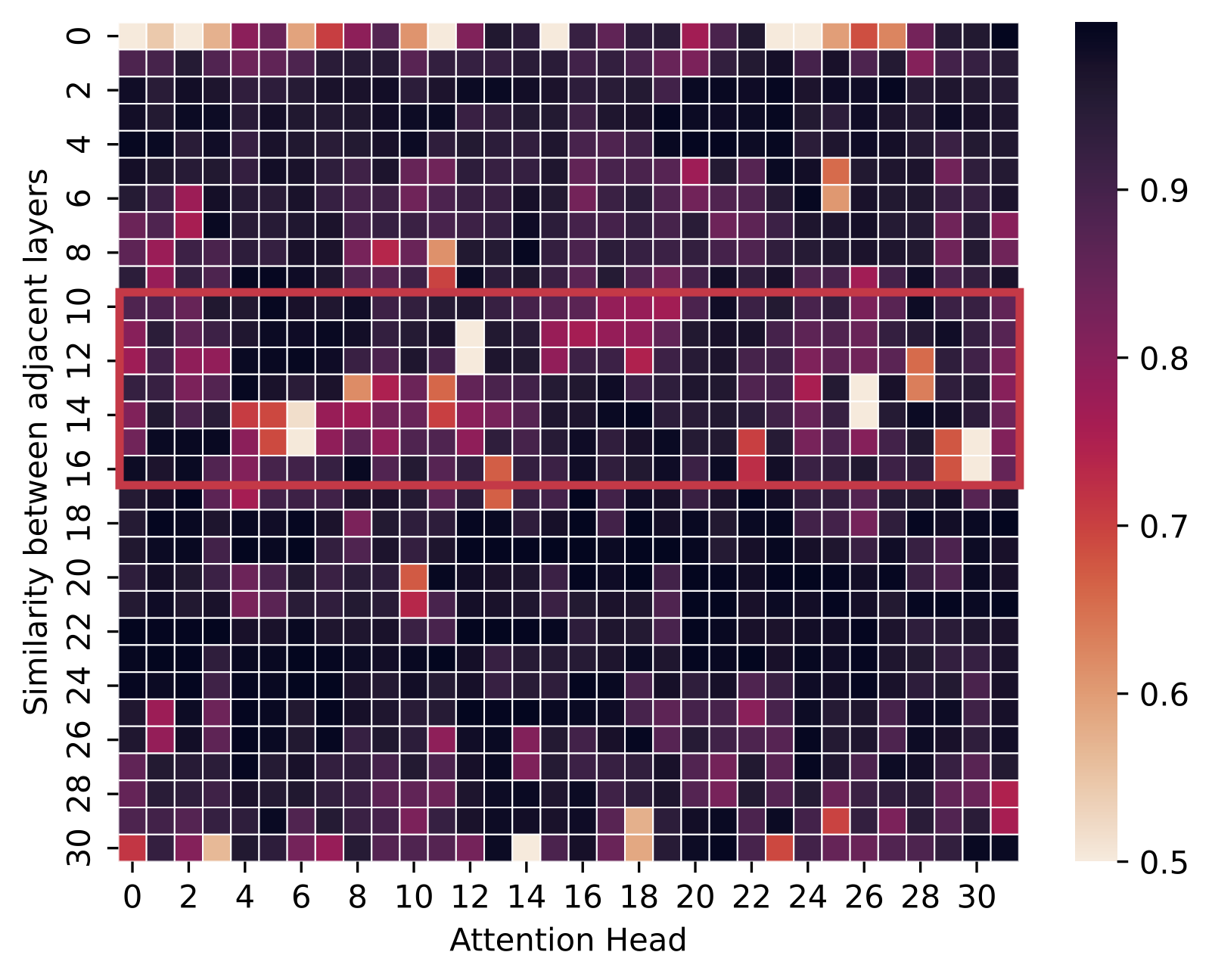
Figure 1. Cosine similarity of the attention scores for adjacent layers. Higher similarity corresponds to a more similar attention score distribution between adjacent layers. The x-axis is the attention head index, and the y-axis corresponds to the correlation between layer \(i\) and layer \(i+1\) for the \(i\)-th entry.

Figure 2. Recall rate by re-selection Layer, defined as the averaged overlap ratio between the tokens selected by TidalDecode and the ground truth ones across all sparse attention layers. Higher recall rate indicates better coverage if the layer has been selected as the token re-selection layer.

We observe that with only one token selection layer at the third layer, the average recall rates are less than 20% as shown in Figure 2. However, as we choose an additional layer 13 to perform re-selection, the average recall rates boost to almost 40% due to the improvement on the token re-selection as shown in Figure 1, where the token re-selection layer lies in the least correlated regions, identified by the red box.

Based on the observation that consecutive layers share a large number of critical tokens, we design position persistent sparse attention to maximally leverage the token overlaps between consecutive Transformer layers to reduce the computation cost for token selection while achieving high predictive performance. Algorithm 1 shows the pseudo-code for interleaving full attention and sparse layers.

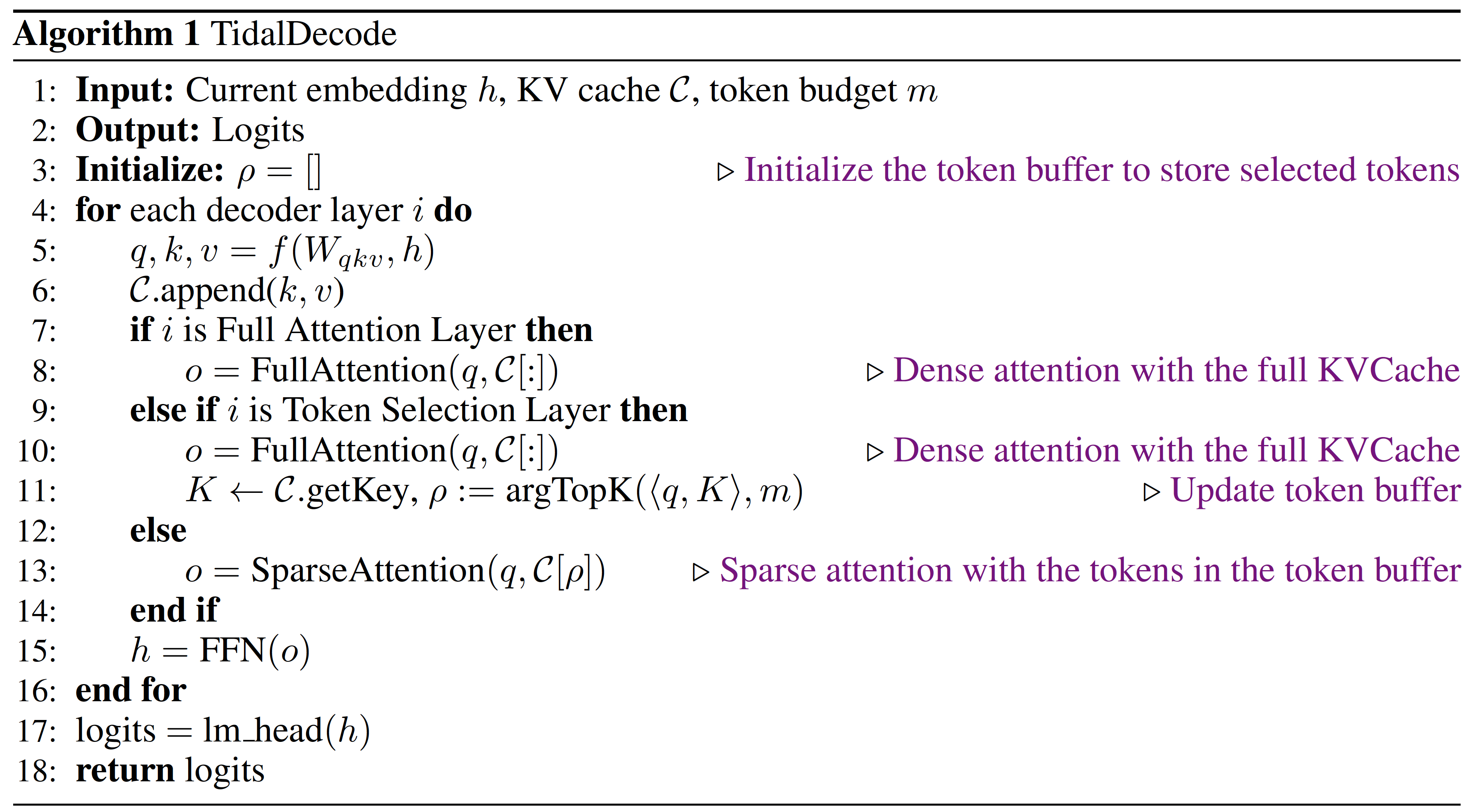
After the initial full attention layers, TidalDecode uses a token selection layer that computes full attention and selects tokens with the highest attention scores. To select tokens, TidalDecode stores the inner product \(\langle q, K \rangle\) on the fly together with full attention calculation. For a given token budget \(m\), TidalDecode then selects the top-\(m\) tokens with the highest inner product values to form a token set \(\rho\). Note that using the inner product to select top-k is equivalent to the post-softmax attention score as the softmax operator is ordering invariant.

All sparse attention layers after a token selection layer compute sparse attention by only loading the keys and values for tokens in \(\rho\), thus limiting the number of tokens participating in attention computations and reducing memory access.

Cache Correction

For tokens decoded by sparse attention methods, their key/value representations can deviate from the original representation of full attention decoded ones, which we refer to as polluted tokens. The problem can be further exacerbated as their KV pairs are added to the KV cache, resulting in the error accumulation or distribution shift of the KV cache. This can lead to model performance drop in scenarios where the generation length is fairly long. To mitigate the KV cache distribution shift issue, TidalDecode uses a cache-correction mechanism, as shown in the following figure, to periodically correct the polluted tokens in the KV cache. For every \(T\) decoding step performed by TidalDecode, there will be a cache correction step through a chunked prefill over all polluted tokens to update their KV representations in the cache. The choice of \(T\) can be at the level of thousands of decoding steps but also depends on different models and tasks. Notice that the cache correction step can be performed concurrently with the sparse decoding step.

Evaluation

In this section, we conduct extensive experiments to assess both the performance and efficiency of TidalDecode. Our evaluations are performed on widely used open-source models, including Llama-2-7B and Llama-3-8/70B. Both models are pretrained decoder-only transformers, exhibiting similar yet distinct architectural features. For TidalDecode, we use TD+Li to denote the TidalDecode using the \(i\)-th layer as the token reselection layer.

Performance Evaluation

Needle-In-The-Haystack The Needle-In-The-Haystack test assesses LLMs’ ability to handle long-dependency tasks, which is particularly critical for sparse attention algorithms. Eviction-based methods (H2O, StreamingLLM) may discard essential tokens, while selection-based approaches (Quest) often fail to consistently identify the ground-truth tokens with the highest attention scores in long contexts.

Since Quest is the current state-of-the-art approach on this task that leverages an estimated attention score on the page level to identify important tokens for sparse attention, we first run TidalDecode on the same test as Quest on the LongChat-7b-v1.5-32k model and obtained results shown in Table 1 with competitive performance.

Table 1. Results of 10k-context-length Needle-In-The-Haystack test on LongChat-7b-v1.5-32k.

To demonstrate the effectiveness of TidalDecode on long-dependency tasks, we further evaluate TidalDecode on tasks with 10K-, 32K-, and 100K-context-window lengths with the Llama-3-70B, Llama-3-8B, Llama-3.1-8B model using the PG-19-mini dataset, shown in Table 2. To ensure fairness, both TidalDecode and Quest use dense attention in the first two layers. In each test, we inserted a random password within the text and tested whether the specific method could retrieve the password correctly.

Table 2. Comprehensive results of 10K-, 32K-, and 100K-context-length Needle-In-The-Haystack test on Llama-3-8B-Instruct-Gradient-1048k, Llama-3.1-8B-Instruct, and Llama-3-70B-Instruct- Gradient-1048k with PG-19-mini dataset.

From Table 2, TidalDecode consistently outperforms Quest and achieves full accuracy with an extremely high sparsity (about 99.5% across all context lengths and models). These results demonstrate TidalDecode can achieve state-of-the-art performance with only two token selection layers. While Quest relies on page-level importance estimation for token selection, TidalDecode’s exact selection with a token reuse approach proves more effective for this task. Also, note that TidalDecode can reduce the token budget by up to 8× when achieving 100% accuracy compared with Quest. This further demonstrates that TidalDecode’s exact token selection layer can obtain more relevant tokens than Quest.

Efficiency Evaluation

To show the efficiency of TidalDecode, we write customized kernels for our approach and measure the end-to-end decoding latency. We conduct evaluation under the configuration of Llama-2-7B on one Nvidia A100 (80 GB HBM, SXM4) with CUDA 12.2. We compare TidalDecode with state-of-the-art full attention serving library FlashInfer and also the Quest implementation. As shown in Figure 3, we can observe that TidalDecode can consistently outperform full attention baseline and Quest by a large margin under all token budgets and context lengths.

TidalDecode achieves this through token pattern reuse to minimize the token selection overhead. Notice that the latest Llama-3 model shares the same architecture as Llama-2, except it uses Group-Query-Attention instead of Multi-Head-Attention. However, this does not affect the relative efficiency comparison against Quest and full attention.

Figure 3. End-to-end latency results on Llama-2-7B model for Full attention baseline(Full), Quest, and TidalDecode(TD) when context length is 10K, 32K, and 100K, respectively. The lower the better.

In Figure 4, we compare the overall attention latency between different methods on the Llama model with 32/64 layers. For the 32-layer Llama model, we have 2 full attention layers + 2 token selection layers + 28 sparse attention layers, while Quest has 2 full attention layers + 30 Quest attention layers. For the 64-layer Llama model, we have 2 full attention layers + 2 token selection layers + 60 sparse attention layers, while Quest has 2 full attention layers + 62 Quest attention layers. Thus, by completely removing the token estimation overhead in the sparse attention layers, for the 32-layer and 64-layer Llama model under all context lengths, TidalDecode can consistently achieve the lowest serving latency while bringing up to 5.56× speed-up ratio against the full attention baseline and 2.17× speed-up ratio against Quest. When the context length is 10K, Quest has a higher latency due to the token selection overhead, which aligns with the end-to-end results in Figure 3. In contrast, TidalDecode still achieves significant speed-up by utilizing the position persistent sparse attention mechanism.

Figure 4. Overall attention latency results for different methods on the LLaMA model with (a) 32 and (b) 64 layers, the lower the better. We use the full attention model as a reference and show TidalDecode and Quest’s overall attention latency ratio. For each group of the bar plots, the left/middle/right bar denotes the full attention baseline, Quest, and TidalDecode, respectively.

Sensitivity Analsys on the Choice of Token-Reselection Layer

We further conduct sensitivity studies for different choices of the token re-selection layer. As TidalDecode only has one token re-selection layer in the middle, it is critical to choose the best-performed one. As shown in Figure 5, we have two interesting findings: (1). Different choices of token re-selection layers can significantly affect the accuracy of the results (2). For models within the same model family, the optimal token re-selection layer is consistent over different tasks. In our setup, the optimal token re-selection layer for the Llama-2-7B model is layer 7, while for the Llama-3-8B/Llama-3.1-8B model is layer 13.

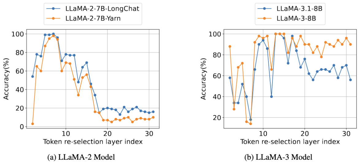
Figure 5: Sensitivity study on the choice of different token re-selection layer. We evaluate LLaMA- 2-7B-LongChat, LLaMA-2-7B-Yarn, LLaMA-3-8B, and LLaMA-3.1-8B with TidalDecode with a token budget of 256 on the Needle-In-The-Haystack task and report their accuracies. The higher the better.

Conclusion

To conclude, this blog introduces TidalDecode, an efficient LLM decoding framework leveraging a novel sparse attention algorithm. On observing the correlation of the pattern of tokens with the highest attention scores across different consecutive layers, TidalDecode proposes only to select tokens twice: once at the beginning layers and once in the middle layer to serve as a token re-selection layer. We find that using two token selection layers is necessary and sufficient to achieve high-generation quality. Additionally, by reusing the token patterns throughout the sparse attention layer, TidalDecode greatly reduces the token selection overhead, resulting in a significant end-to-end speed-up ratio against existing methods. More interestingly, the optimal choice of the token re-selection layer is consistent across different tasks if the model is in the same model family.