Table of Contents
1. Motivation
2. Purpose
3. Overview
4. Preface
4.1 Linear Layers
5. The Calculation
5.1 Convolutional Filters
5.2 Pooling Filters
6. The Initial Conditions
6.1 Input Channels
7. Parameter Definition
7.1 Kernel (Filter) Size
7.2 Output Channels
7.3 Bias Term
8. The Manipulation
8.1 Padding
8.2 Dilation
9. The Application
9.1 Stride
9.2 Groups
10. Other Specifications
10.1 Padding Modes
10.2 Return Indices
10.3 Ceiling Mode
11. Additional Resources
1. Motivation
In the previous assignment, you learned how to interpret fully connected neural networks such as Multilayer Perceptrons (MLPs). Much attention was needed to understand the tradeoff between bias and variance, where a variety of methods were proposed to reduce overfitting, e.g. batch normalization, reducing complexity, etc. Here, you will be learning a different approach to the fully connected interpretation, where we view data as having patterns from which we can hierarchically derive more and more convolved representations -- that is, convolutional neural networks (CNNs).
CNNs utilize convolutional and pooling layers, among others. These models rely heavily on the notion that filters (also known as kernels) and their operations are able to extract higher-level features (also known as patterns). In other words, given a set of low-level features, we are able to infer a set of higher level features from which it is easier for us to do classification or prediction. From layer to layer, we can hierarchically use lower level features to create higher-level features, culminating with a model whose structure consists of a hierarchical pattern whose features were extracted using filters.
The use of filters in CNNs has multiple implications. First, in assuming patterns can be extracted from scanning an image, it is a necessary consequence that those patterns can be recognized anywhere in the image. When filters are “shifted” during their usage to derive parameters, we term the resulting benefit as shift invariance. Models that are shift invariant are able to recognize patterns anywhere in an image, regardless of (i.e. invariant to) where the pattern is located.
In PyTorch, the terms “filter” and “kernel” are used interchangeably. However, in the literature, a kernel is a filter with a convolution applied. As such, it does not make sense to apply pooling to a kernel (since it is the necessary application of convolution), rather we would say you apply pooling to a filter.
2. Purpose
The purpose of this reference is to facilitate an understanding of the core concepts behind the classes and algorithms you will be deriving from scratch or utilizing in the PyTorch framework. In this regard, there are four classes you must understand at a minimum and will see very often in a variety of neural network architectures.
For Homework 2 Part 2:
torch.nn.Conv2d(in_channels, out_channels, kernel_size, stride=1, padding=0, dilation=1, groups=1, bias=True, padding_mode='zeros')
Documentation: https://pytorch.org/docs/stable/nn.html#conv2d
torch.nn.MaxPool2d(kernel_size, stride=None, padding=0, dilation=1, return_indices=False, ceil_mode=False)
Documentation: https://pytorch.org/docs/stable/nn.html#torch.nn.MaxPool2d
For Homework 2 Part 1:
torch.nn.Conv1d(in_channels, out_channels, kernel_size, stride=1, padding=0, dilation=1, groups=1, bias=True, padding_mode='zeros')
Documentation: https://pytorch.org/docs/stable/nn.html#id21
torch.nn.MaxPool1d(kernel_size, stride=None, padding=0, dilation=1, return_indices=False, ceil_mode=False)
Documentation: https://pytorch.org/docs/stable/nn.html#maxpool1d
There are variants of these classes, but these will serve as fundamental references.
3. Overview
First, you must understand the difference between these two types of operations:
Further, you must understand the meaning, motivation, and results expected when using the following arguments:
These are all in the provided documentation, which is very well written and you are expected to understand.
To supplement the documentation, we have created examples of how changing the arguments of the specified classes results in a change to one of five properties:
4. Preface
So far, we have talked about multilayer perceptrons (MLPs), so you should understand how a linear mapping of inputs to outputs is done in PyTorch. Further, you should know what it means to have a bias term and the difference between a bias term versus an input that was previously an output followed by an activation. That is, you should understand the following:
torch.nn.Linear(in_features, out_features, bias=True)
Reference: https://pytorch.org/docs/stable/nn.html#linear
5. The Calculation
5.1 Convolutional Filters
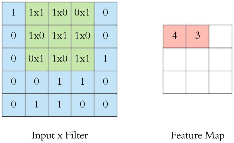
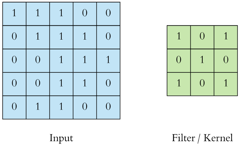
Convolution is nothing but a mathematical operation that merges two sets of information. In the case of a CNN, convolutions are performed on the input data with the use of a filter or kernel to then produce a feature map. The convolution is executed by sliding the filter over the input and performing dot products between the filters and local regions of the input. Consider the illustrative example below:
Figure 1: input and kernel
In Figure 1 above, on the left, we have an input to the convolutional layer in the form of an input image, for example. On the right we have the convolution filter/kernel of size 3x3 (i.e. width = 3 and height = 3). We do the convolution by sliding this filter over the input. At every location, we do element-wise matrix multiplication and then sum the result to get a single value. This value goes into the feature map. This operation is shown in Figure 2 below.
Figure 2: Single step in the convolution operation
The green area where the convolution takes place is called the receptive field. Due to the size of the filter, the receptive field is also 3x3. Here the filter is at the top left and the output of the convolution operation is 4 because: (1x1) + (1x0) + (1x1) + (0x0) + (1x1) + (1x0) + (0x1) + (0x0) + (1x1) = 4. We then slide the filter from left to right and perform the same operation, adding that result to the feature map as well (see Figure 3 below).
Figure 3: Another single step in the convolution operation
We keep doing this and collect the convolution results in the feature map. Figure 4 below is an animation that shows the entire convolution operation. Figure 5 shows the same operation but shows the input, the filter and the feature map in 3D. We have seen how the basic convolution operation works. You can use the following resources for additional information:
An Intuitive Guide to CNNs:
https://www.freecodecamp.org/news/an-intuitive-guide-to-convolutional-neural-networks-260c2de0a050/
Visualizing Convolutions in Multiple Channels:
http://cs231n.github.io/convolutional-networks/#overview
https://mlnotebook.github.io/post/CNN1/
Step-by-step Convolution Operation:
Convolution in action:
http://setosa.io/ev/image-kernels/
Figure 4: On the Left, the filter slides over the input.
On the Right, the result is summed and added to the feature map.
Figure 5: Convolution operation
5.2 Pooling Filters
One limitation of the feature map output of convolutional layers is that they capture the exact position of features in the input. This means that small movements in the position of the feature in the input image will result in a different feature map. This can happen with re-cropping, rotation, shifting, and other minor changes to the input image.
In all cases, pooling helps to make the representation approximately invariant to small translations of the input. Invariance to translation means that if we translate the input by a small amount, the values of the pooled outputs do not change. This property of invariance to translation can be useful if we care more about whether some feature is present than exactly where it is.
A pooling layer is a new layer added after the convolutional layer. Specifically, after a nonlinearity (e.g. ReLU) has been applied to the feature maps output by a convolutional layer; for example, the layers in a model may look as follows:
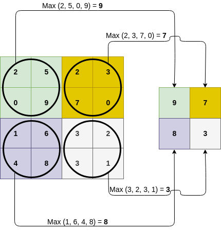
The pooling layer operates upon each feature map separately to create a new set of the same number of pooled feature maps. The size of the pooling operation or filter is smaller than the size of the feature map. Commonly used pooling filter size is 2x2 with a stride of 2. This means that the pooling layer will always reduce the size of each feature map by a factor of 2, e.g. each dimension is halved, reducing the number of pixels or values in each feature map to one quarter the size (see example below).
Types of pooling include max pooling (maximum output within a rectangular neighborhood), average pooling (average of a rectangular neighborhood), L2-norm pooling (L2-norm of a rectangular neighborhood), or a weighted average based on the distance from the central pixel. Figure 6 below shows an example of max pooling operation (the arrows) applied to the feature maps output by a convolutional layer with a stride of 2 (left: 4x4 sized input) resulting in pooled feature map output (right: 2x2 sized output).
Figure 6: Max Pooling operation
You are encouraged to review the following materials to get more insight on this topic:
Visualizing Pooling:
https://www.youtube.com/watch?time_continue=23&v=_Ok5xZwOtrk
Pooling operation:
https://www.youtube.com/watch?v=8oOgPUO-TBY
6. The Initial Conditions
6.1 Input Channels
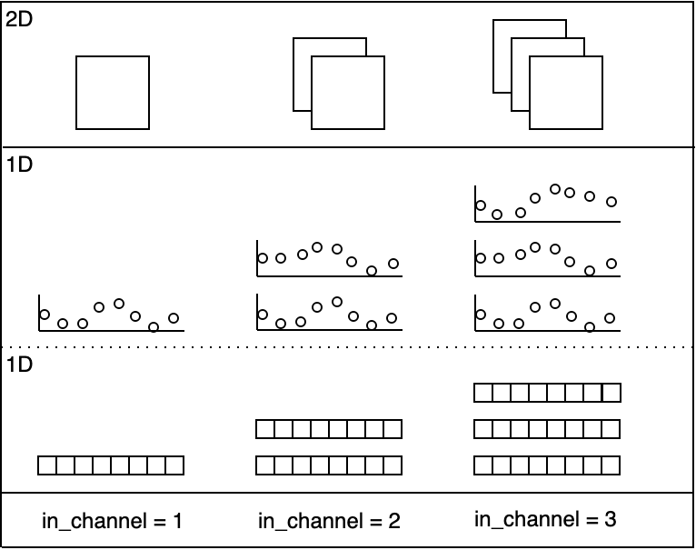
in_channels: Input channels are those which are provided as an input to a layer. For 2D inputs to the first layer, typical measurements include grayscale (1 channel), RGB (3 channels), and CMYK (4 channels). For 1D inputs to the first layer, typical measurements include polysomnogram (12 channels), WLAN (14 channels), and RAS-24 (24 channels). As will be discussed, each kth layer is followed by a set of output channels and these will be the input channels to the (k+1)th layer.
Figure 7: Visualization of changes in the in_channel parameter value.
7. Parameter Definition
7.1 Kernel (Filter) Size
kernel_size: As the name indicates, kernel_size specifies the size of the kernel to be used for convolution. Figure 7 below shows different kernel sizes both for 2D and 1D convolution.
Figure 8: Visualizations of changes in the kernel sizes parameter value.
7.2 Output Channels (Number of Filters)
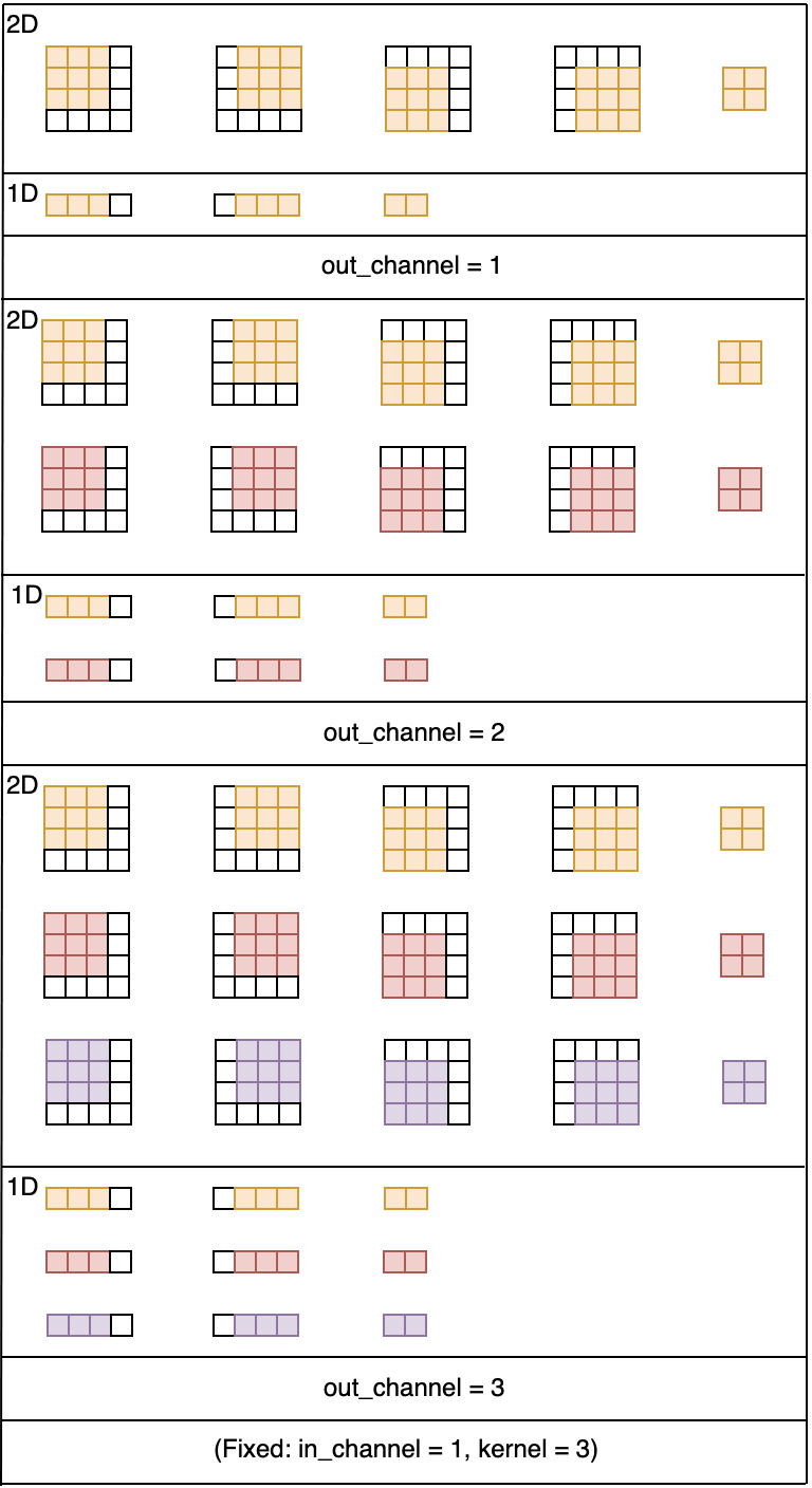
out_channel: Output channels are exactly the same as the number of filters used. In other words, if you want to specify the number of filters you would like to use, it should be specified using the out_channel parameter. For each filter, you will scan the data from left to right and up to down. The result of each individual scan will yield a parameter whose result depends on if you used a convolutional or pooling operation.
Figure 9: Visualization of changes to the out_channel parameter value.
The number of input channels and the kernel size are fixed.
7.3 Bias Term
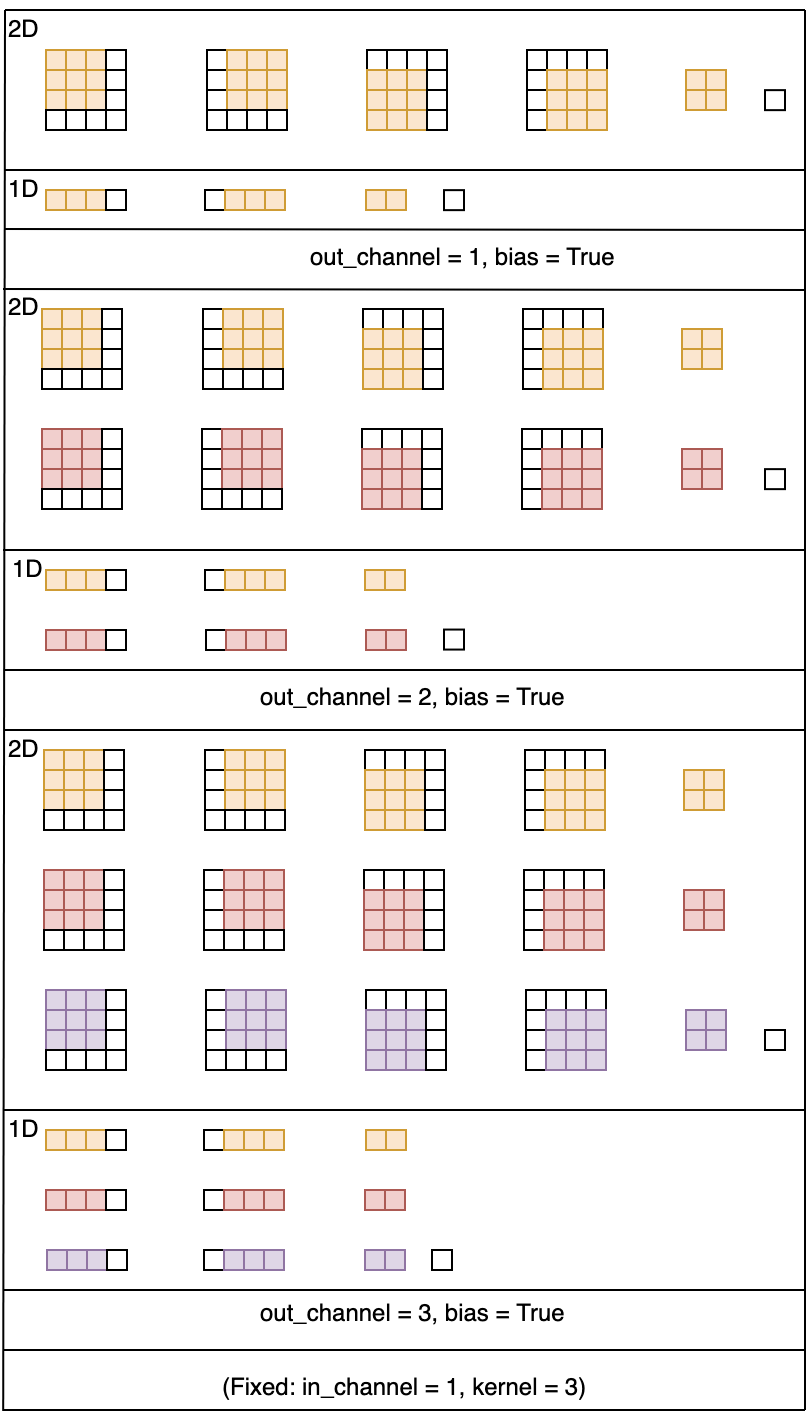
bias: Bias in a convolutional layer is a unique scalar value which is added to the output of a convolution at every single pixel. Figure 10 below illustrates where a bias is added.
Figure 10: Bias in a convolutional layer
Figure 11: Visualization of adding bias parameter value.
Notice the similarity to Figure 9, with one bias for each set of channels.
8. The Manipulation
8.1 Padding
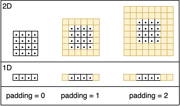
padding: Padding is used to increase an input’s dimension, which is best demonstrated by means of an example. Please refer to the documentation to understand what types of padding values are available.
Figure 12: Visualization of changes to the padding parameter value.
8.2 Dilation
dilation: Dilation is an alternative to padding, which is also best demonstrated by means of an example. Please refer to the documentation to understand what types of dilation values are available.
Figure 13: Visualization of changes to the dilation parameter value.
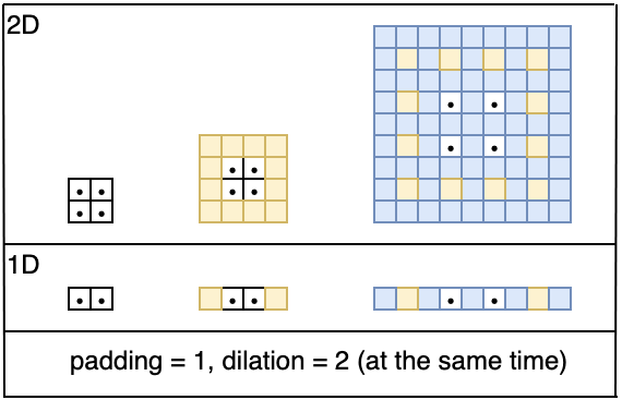
Note: It is worth noting that both padding and dilation can be specified. If you decide to specify both, PyTorch will first pad then dilate the image.
Figure 14: Visualization of specifying a change to the padding parameter and
the dilation parameter. The result of such a specification is the rightmost visual.
9. The Application
9.1 Stride
stride: We must specify the Stride with which we slide the filter. Stride is simply the number of pixels in the feature map by which the filter is slid both across the width and height (for 2D convolution) or just across the width (for 1D convolution) of the input feature map during convolution. I.e. For example, for 2D convolution, when the stride is 1 then we move the filters one pixel at a time. When the stride is 2 then the filters jump 2 pixels at a time as we slide them around. Example 6, 7, and 8 below show a 2D convolution with different strides. The same thing can be generalized for 1D as it is similar to 2D convolution except the convolution is only in one dimension. The blue grid represents the feature map and the magenta represents the output of the convolution. Notice how the strides determines the size of the output feature map. In addition to the stride of the convolution, padding and filter size also determine the size of the output.
The following formula can be used to compute the size of the output of the convolution both for 1D and 2D convolutions:
For 2D convolution:
Where the corresponding variables:
For 1D convolution:
You can confirm the results from the animations below using the formula.
Figure 15: Visualization of Strides
Filter size (F) 3×3
Stride (S): 1
Padding: 0
Input feature map size ( Wi × Hi ): 4×4
Output size ( W0 × H0 ): 2×2
Figure 16: Visualization of Strides
Filter size (F) 3×3
Stride (S): 2
Padding (P): 0
Input feature map size ( Wi × Hi ): 5 × 5
Output size ( W0 × H0 ): 2 × 2
Figure 17: Visualization of Strides
Filter size (F) of 5×5
Stride: 4, padding (P): 0,
Input feature map size ( Wi × Hi ): 13×13,
Output size ( W0 × H0 ): 3×3
Resources relevant to this topic:
Convolution arithmetic:
https://arxiv.org/pdf/1603.07285.pdf
9.2 Groups
groups: Groups are used to group sets of inputs, as seen in the following examples.
Figure 18: Visualization of the default group parameter specification of 1.
Figure 19: Visualization of the group parameter specification of 2.
Figure 20: Visualization of the group parameter specification of 3.
10. Other Specifications
See documentation for the meaning and usage of padding_mode, return_indices, and ceil_mode.
11. Convolution example
Figure 21 below shows an example convolutional layer together with the values that the parameters of the Conv2D class should take.
in_channel = 3
out_channel = 2
kernel_size = (3,3)
stride = 2
padding = 1
dilation = 1
groups = 1
bias = true
Padding_mode = zeros
Figure 21 convolution example
12. Additional Resources