PDE Constrained Optimization: Slides

Outline

What is the Inverse Problem?
A theoretic framework for solving PDECO
The eikonal equation

The Forward Problem

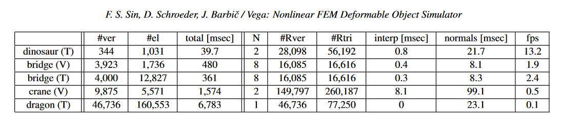
Solving a physical problem requires simulation

\mathcal{S}(x ; \theta) = 0

\mathcal{S}(x ; \theta) = 0

Given parameters, $\theta$ , what is a configuration, $x$ , that satisfies the above equation?

The Forward Problem

Examples of $\theta$ :

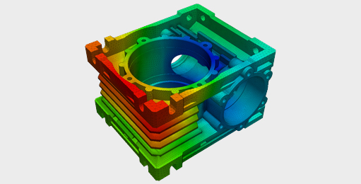
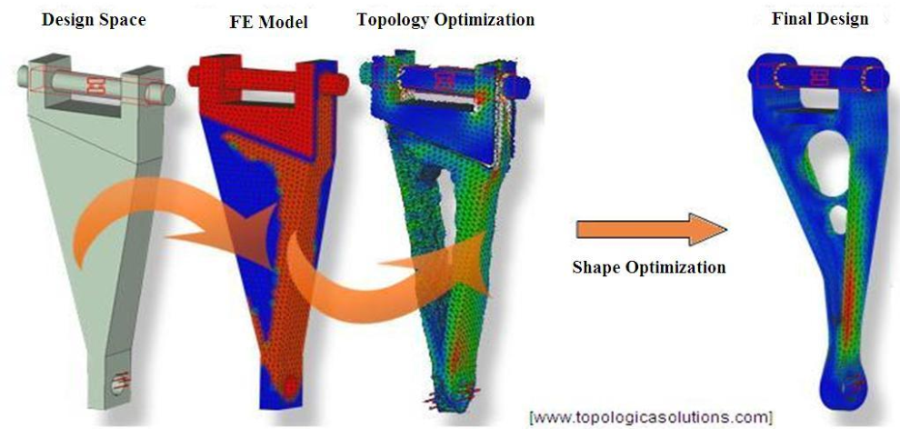
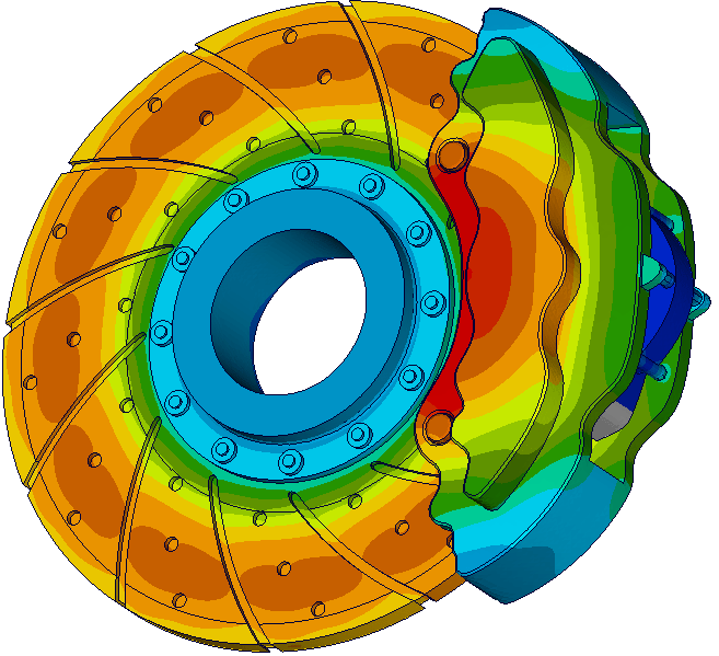
Surface shape for FEM
Initial conditions for the simulation
Resistance parameter for traveling waves

Configuration could refer to the heat value at a particular time, or the position at a time value.

The Inverse Problem

"I want to find the parameters, $\theta$ , that will admit the configuration, $x$ , that I observed/desire"

\underset{\theta}{\text{min}} {\displaystyle \int} \left(x - x_{observed} \right)^2

\underset{\theta}{\text{min}} {\displaystyle \int} \left(x - x_{observed} \right)^2

s.t. ~~\mathcal{S}(x; \theta) = 0

s.t. ~~\mathcal{S}(x; \theta) = 0

The Inverse Problem

Examples include:

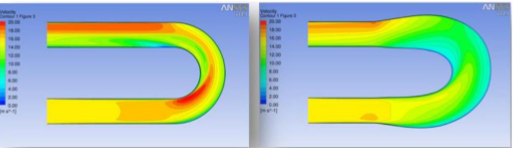
Shape Optimization
- Stress
- Fluid Control
- etc.
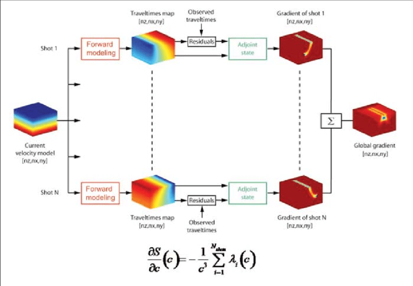
Seismic Imaging
- Wave modeling
- Traveltime modeling

The inverse optimization problem is hard.

Each evaluation of the loss function requires a full simulation. To calculate a gradient, finite difference would require multiple runs of the same simulation.

The inverse optimization problem is functional.

PDEs are described in terms of function spaces. Consequently, the inverse problem is also in terms of function spaces rather than discrete vector spaces

The optimization will be effected by our choice of discretization

How to solve PDECO?

\lVert \nabla \Phi \rVert = \eta

\lVert \nabla \Phi \rVert = \eta

There's no one-size-fits-all solution!

\frac{\partial \mathbf{u}}{\partial t} + (\mathbf{u} \cdot \nabla) \mathbf{u} - \nu \,\nabla^2 \mathbf{u} = - \nabla w + \mathbf{g}

\frac{\partial \mathbf{u}}{\partial t} + (\mathbf{u} \cdot \nabla) \mathbf{u} - \nu \,\nabla^2 \mathbf{u} = - \nabla w + \mathbf{g}

\frac{\partial u}{\partial t} = \frac{\partial^2 u}{\partial x^2}

\frac{\partial u}{\partial t} = \frac{\partial^2 u}{\partial x^2}

Building a theory

\underset{\theta}{\text{min}}~ f(x)

\underset{\theta}{\text{min}}~ f(x)

s.t. ~~\mathcal{S}(x; \theta) = 0

s.t. ~~\mathcal{S}(x; \theta) = 0

We need $d_{\theta}f$ in order to do any gradient based optimization

\underset{\theta}{\text{min}}~ f(x(\theta))

\underset{\theta}{\text{min}}~ f(x(\theta))

s.t. ~~\mathcal{S}(x(\theta); \theta) = 0

s.t. ~~\mathcal{S}(x(\theta); \theta) = 0

Calculating $d_\theta f$

d_\theta f(x(\theta)) = d_x f \cdot d_\theta x

d_\theta f(x(\theta)) = d_x f \cdot d_\theta x

d_\theta \mathcal{S}(x(\theta); \theta) = 0

d_\theta \mathcal{S}(x(\theta); \theta) = 0

d_\theta x = - d_x \mathcal{S}^{-1} \cdot d_\theta \mathcal{S}

d_\theta x = - d_x \mathcal{S}^{-1} \cdot d_\theta \mathcal{S}

d_\theta f(x(\theta)) = d_x f \cdot - d_x \mathcal{S}^{-1} \cdot d_\theta \mathcal{S}

d_\theta f(x(\theta)) = d_x f \cdot - d_x \mathcal{S}^{-1} \cdot d_\theta \mathcal{S}

Calculating $d_\theta f$

d_\theta f(x(\theta)) = d_x f \cdot - d_x \mathcal{S}^{-1} \cdot d_\theta \mathcal{S}

d_\theta f(x(\theta)) = d_x f \cdot - d_x \mathcal{S}^{-1} \cdot d_\theta \mathcal{S}

(d_x \mathcal{S})^T \lambda = -(d_x f)^T

(d_x \mathcal{S})^T \lambda = -(d_x f)^T

Derivative of dynamics

(application specific)

Derivative of cost functional

(closed form usually)

\lambda^T

\lambda^T

}

The Adjoint State

(d_x \mathcal{S})^T \lambda = -(d_x f)^T

(d_x \mathcal{S})^T \lambda = -(d_x f)^T

$\lambda$ is known as the adjoint state

$\lambda$ is the same dimension as the configuration, $x$ .

Solving for the adjoint state is no harder than running the forward simulation; it is often a linear solve

Lagrange Multipliers

The adjoint state can be derived from Lagrange multipliers.

s.t. ~~\mathcal{S}(x; \theta) = 0

s.t. ~~\mathcal{S}(x; \theta) = 0

\underset{\theta}{\text{min}}~ f(x)

\underset{\theta}{\text{min}}~ f(x)

\underset{\theta}{\text{min}}~ f(x^*) + \lambda^* \mathcal{S}(x; \theta)

\underset{\theta}{\text{min}}~ f(x^*) + \lambda^* \mathcal{S}(x; \theta)

where $x^*$ and $\lambda^*$ are critical points.

Lagrange Multipliers

One can view the adjoint state method as an extension of discrete Lagrange multipliers to functionals, where $\lambda$ is a function instead of a coefficient.

In the PDECO literature, the KKT conditions are referenced a lot in the context of functional analysis.

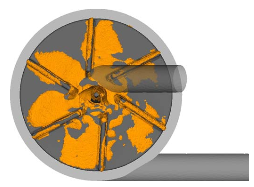
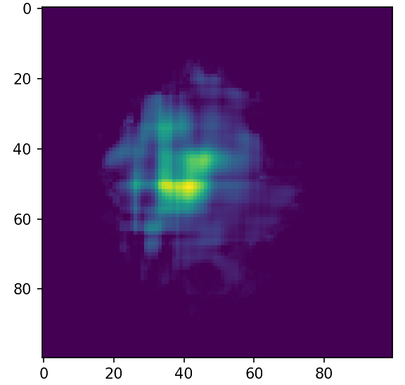
The eikonal as an example

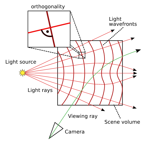
From images of a volume, and I want to invert the image formation model to obtain the volume. Our equation of interest is the eikonal equation

The eikonal as an example

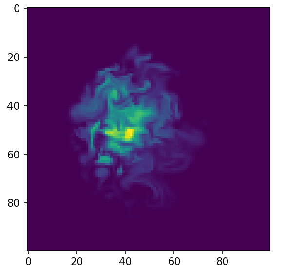
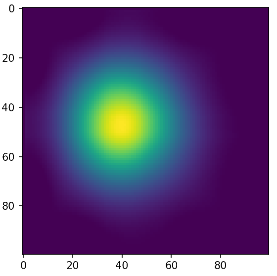
Ground Truth

Initialization

Adjoint

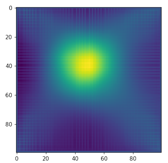
The eikonal as an example

Ground Truth

Initialization

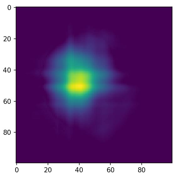
Step 3

Final

Out of the box optimization gives good results!

Conclusion

PDE Constrained Optimization is Lagrange Multipliers in disguise
The broad theory for the adjoint state method can be used to tackle inverse problems
Generally, the adjoint is faster to solve than the forward simulation itself

References and Links

Nice explanation of the derivation:
- https://cs.stanford.edu/~ambrad/adjoint_tutorial.pdf
Presentation on Cea's Method for shape optimization:
- https://www.ljll.math.upmc.fr/frey/cours/EAFIT/shapeOptim.pdf
Generally, the adjoint is faster to solve than the forward simulation itself

PDE Constrained Optimization

Solving Inverse Problems

Arjun Teh

Outline

The Forward Problem

The Forward Problem

The Inverse Problem

The Inverse Problem

The inverse optimization problem is hard.

The inverse optimization problem is functional.

How to solve PDECO?

Building a theory

Calculating $d_\theta f$

Calculating $d_\theta f$

The Adjoint State

Lagrange Multipliers

Lagrange Multipliers

The eikonal as an example

The eikonal as an example

The eikonal as an example

Conclusion

References and Links