Inverting the Eikonal Equation

Using PDE-Constrained Optimization

Arjun Teh

Outline

  • The eikonal equation and its inverse
  • Solving the inverse problem
  • The discrete version

The Eikonal Equation

Scenarios with eikonal

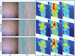
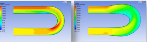
  • Gas Flow Reconstruction
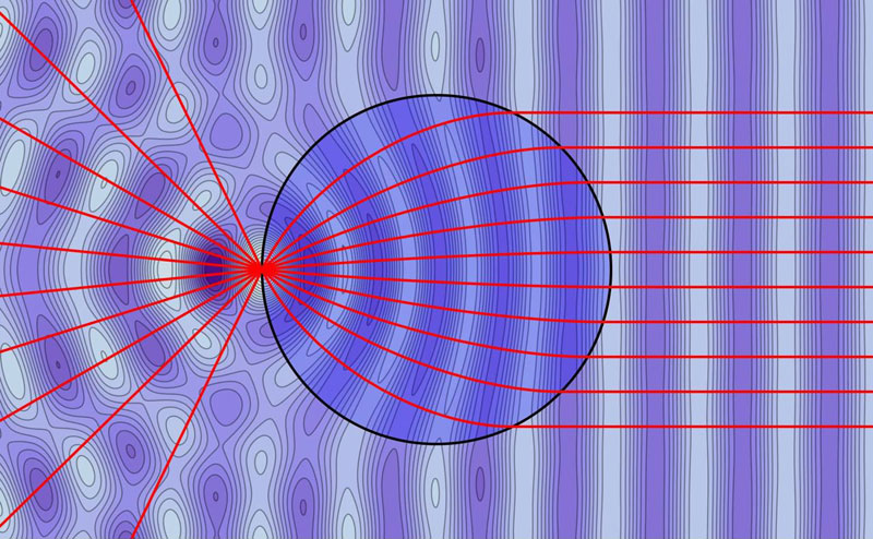
  • GRIN Lens

Describes the geometric properties of a wave with small wavelength moving through a medium

The Forward Problem

The eikonal equation is a PDE

\lVert \nabla \Phi \rVert^2 = \eta^2

Given a refractive index field, \(\eta\), what is a configuration, \(\Phi\), that satisfies the above equation?


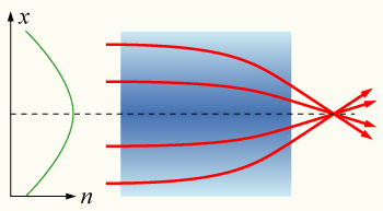
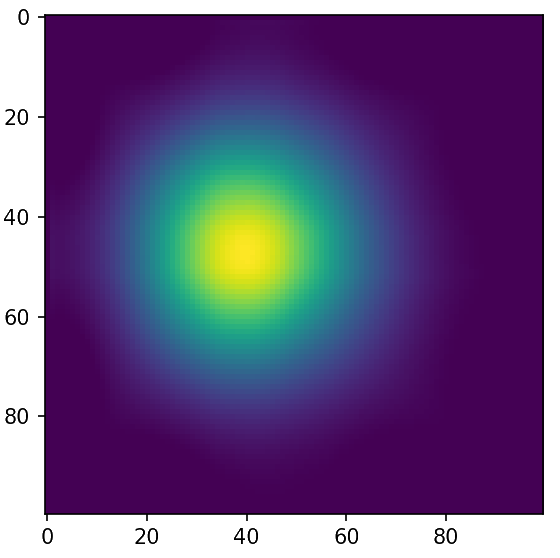
\(\Phi\) is the phase of the wavefront, and \(\nabla \Phi \) describes how rays will propagate through the volume

The Forward Problem

The eikonal equation can be solved in different ways

  • Fast Marching (wave propagation)
  • Raytracing (ray marching)

All of them solve for the phase (\(\Phi\)) given the underlying refractive field (\(\eta\))

The Inverse Problem

"I want to find the refractive field, \(\eta\), that will admit the configuration, \(\Phi\), that I observed/desire"

\underset{\eta}{\text{min}} {\displaystyle \int_{d\Omega}} \left(\Phi - \Phi_{observed} \right)^2
s.t. ~~\lVert \nabla \Phi \rVert^2 - \eta^2 = 0

Reframe the optimization

\underset{\eta}{\text{min}} {\displaystyle \int_{d\Omega}} \left(\Phi - \Phi_{observed} \right)^2
s.t. ~~\lVert \nabla \Phi \rVert^2 - \eta^2 = 0
\underset{\eta, \lambda, \Phi}{\text{min}} ~~\mathcal{C}(\eta)
- {\displaystyle \int_{\Omega}} \lambda \left( \lVert \nabla \Phi \rVert^2 - \eta^2 \right)
\mathcal{C}(\Phi(\eta))

Reframe the optimization

\underset{\eta, \lambda, \Phi}{\text{min}} ~~\mathcal{C}(\Phi(\eta))
- {\displaystyle \int_{\Omega}} \lambda \left( \lVert \nabla \Phi \rVert^2 - \eta^2 \right)
\mathcal{L}(\eta, \lambda, \Phi)

With this formulation, we can conceptually treat \(\eta, \lambda,\) and \(\Phi\) as independent variables.

If we want to do gradient descent, our new optimization problem will be equivalent to our original problem if we insist that \(\lambda\) and \(\Phi\) are critical points of \(\mathcal{L}\).

Reframe the optimization

\frac{d}{d\eta}\mathcal{C}(\Phi(\eta)) = \frac{d}{d\eta}\mathcal{L}(\eta, \lambda^*, \Phi^*)
\frac{d\mathcal{L}(\eta, \lambda^*, \Phi^*)}{d\lambda} = \frac{d\mathcal{L}(\eta, \lambda^*, \Phi^*)}{d\Phi} = 0

where,

Finding \(\Phi^*\)

\mathcal{L} = \mathcal{C}(\Phi) - {\displaystyle \int_{\Omega}} \lambda \left( \lVert \nabla \Phi \rVert^2 - \eta^2 \right)
\frac{d\mathcal{L}}{d\lambda} = - {\displaystyle \int_{\Omega}} \left( \lVert \nabla \Phi \rVert^2 - \eta^2 \right) = 0

Solving the original forward problem yields a critical point with respect to \(\lambda\).

Finding \(\lambda^*\)

\mathcal{L} = \mathcal{C}(\Phi) - {\displaystyle \int_{\Omega}} \lambda \left( \lVert \nabla \Phi \rVert^2 - \eta^2 \right)
\frac{d\mathcal{C}}{d\Phi} - \frac{d}{d\Phi}{\displaystyle \int_{\Omega}} \lambda \left( \lVert \nabla \Phi \rVert^2 - \eta^2 \right) = 0

Assuming we have \(\Phi\), we can solve for \(\lambda\)

\frac{d\mathcal{L}}{d\Phi} =

Finding \(\lambda^*\)

\frac{d\mathcal{C}}{d\Phi} - \frac{d}{d\Phi}{\displaystyle \int_{\Omega}} \lambda \left( \lVert \nabla \Phi \rVert^2 - \eta^2 \right) = 0
\frac{d\mathcal{C}}{d\Phi} - {\displaystyle \int_{\Omega}} \lambda \frac{d}{d\Phi} \left( \lVert \nabla \Phi \rVert^2 - \eta^2 \right) = 0
\frac{d\mathcal{C}}{d\Phi} - {\displaystyle \int_{\Omega}} \lambda \frac{d}{d\Phi} \lVert \nabla \Phi \rVert^2 = 0

Finding \(\lambda^*\)

\frac{d\mathcal{C}}{d\Phi} - {\displaystyle \int_{\Omega}} \lambda \frac{d}{d\Phi} \lVert \nabla \Phi \rVert^2 = 0
\frac{d\mathcal{C}}{d\Phi} - {\displaystyle \int_{\Omega}} \lambda 2\left( \nabla \Phi \right)^T \left(d\nabla \Phi\right) = 0
\frac{d\lVert x \rVert^2}{dx} = 2x^T
\frac{d\mathcal{C}}{d\Phi} - {\displaystyle \int_{\Omega}} \lambda 2\left( \nabla \Phi \right)^T \left(\nabla d\Phi\right) = 0

Finding \(\lambda^*\)

\frac{d}{d\Phi} {\displaystyle \int_{\partial\Omega}} \left(\Phi - \hat{\Phi}\right)^2 - 2{\displaystyle \int_{\Omega}} \lambda \left( \nabla \Phi \right)^T \left(\nabla d\Phi\right) = 0
{\displaystyle \int_{\partial\Omega}} 2\left(\Phi - \hat{\Phi}\right)d\Phi - 2{\displaystyle \int_{\Omega}} \lambda \left( \nabla \Phi \right)^T \left(\nabla d\Phi\right) = 0
\frac{d\mathcal{C}}{d\Phi} - {\displaystyle \int_{\Omega}} \lambda 2\left( \nabla \Phi \right)^T \left(\nabla d\Phi\right) = 0

Finding \(\lambda^*\)

{\displaystyle \int_{\partial\Omega}} 2\left(\Phi - \hat{\Phi}\right)d\Phi - 2{\displaystyle \int_{\Omega}} \lambda \left( \nabla \Phi \right)^T \left(\nabla d\Phi\right) = 0
{\displaystyle \int_{\Omega}} \nabla u^T \mathbf{F} = {\displaystyle \int_{\partial\Omega}} u\left( \mathbf{F}^T \mathbf{\hat{n}}\right) - {\displaystyle \int_{\Omega}} u(\nabla \cdot \mathbf{F})
\mathbf{F} = \lambda \nabla \Phi
u = d\Phi

Using Divergence Theorem:

{\displaystyle \int_{\partial\Omega}} \left(\lambda \nabla \Phi\right)^T \mathbf{\hat{n}} d\Phi - {\displaystyle \int_{\Omega}} \nabla \cdot \lambda \left( \nabla \Phi \right) d\Phi

Finding \(\lambda^*\)

{\displaystyle \int_{\partial\Omega}} 2\left(\Phi - \hat{\Phi}\right)d\Phi - 2{\displaystyle \int_{\Omega}} \lambda \left( \nabla \Phi \right)^T \left(\nabla d\Phi\right) = 0
0 = {\displaystyle \int_{\partial\Omega}} \left(\Phi - \hat{\Phi}\right)d\Phi \\ - \left({\displaystyle \int_{\partial\Omega}} \left(\lambda \nabla \Phi\right)^T \mathbf{\hat{n}} d\Phi - {\displaystyle \int_{\Omega}} \nabla \cdot \lambda \left( \nabla \Phi \right) d\Phi \right)

Finding \(\lambda^*\)

0 = {\displaystyle \int_{\partial\Omega}} \left(\Phi - \hat{\Phi}\right) d\Phi\\ - \left({\displaystyle \int_{\partial\Omega}} \left(\lambda \nabla \Phi\right)^T \mathbf{\hat{n}} d\Phi - {\displaystyle \int_{\Omega}} \nabla \cdot \lambda \left( \nabla \Phi \right) d\Phi \right)
{\displaystyle \int_{\partial\Omega}} \left(\Phi - \hat{\Phi}\right) d\Phi - {\displaystyle \int_{\partial\Omega}} \left(\lambda \nabla \Phi\right)^T \mathbf{\hat{n}} d\Phi = 0
{\displaystyle \int_{\Omega}} \nabla \cdot \lambda \left( \nabla \Phi \right) d\Phi = 0

Finding \(\lambda^*\)

{\displaystyle \int_{\partial\Omega}} \left(\Phi - \hat{\Phi}\right)d\Phi - {\displaystyle \int_{\partial\Omega}} \left(\lambda \nabla \Phi\right)^T \mathbf{\hat{n}} d\Phi = 0
{\displaystyle \int_{\Omega}} \nabla \cdot \lambda \left( \nabla \Phi \right) d\Phi = 0

In order for both of these equations to be true, they need to be true for the whole domain of the integral

Finding \(\lambda^*\)

\left(\Phi - \hat{\Phi}\right) = \left(\lambda \nabla \Phi\right)^T \mathbf{\hat{n}}; ~\text{on}~ \partial \Omega
\nabla \cdot \lambda \left( \nabla \Phi \right)= 0; ~\text{on}~ \Omega

This is known as the adjoint equation, and \(\lambda\) is referred to as the adjoint state.

Recap so far

\frac{d\mathcal{L}}{d\lambda} = 0
{\displaystyle \int_{\Omega}} \left( \lVert \nabla \Phi \rVert^2 - \eta^2 \right) = 0
\frac{d\mathcal{L}}{d\Phi} = 0
\left(\Phi - \hat{\Phi}\right) = \left(\lambda \nabla \Phi\right)^T \mathbf{\hat{n}}; ~\text{on}~ \partial \Omega
\nabla \cdot \lambda \left( \nabla \Phi \right)= 0; ~\text{on}~ \Omega

Forward System

Adjoint System

The Adjoint State

We now know \(\Phi^*\) and \(\lambda^*\) by solving for the stationary points.

\mathcal{L} = {\displaystyle \int_{\partial\Omega}} (\Phi - \hat{\Phi})^2 - {\displaystyle \int_{\Omega}} \lambda \left( \lVert \nabla \Phi \rVert^2 - \eta^2 \right)
\frac{d}{d\eta}\mathcal{L} = {\displaystyle \int_{\Omega}} \lambda \left( - \frac{d}{d\eta}\eta^2 \right)

The Adjoint State

We now know \(\Phi^*\) and \(\lambda^*\) by solving for the stationary points.

\frac{d}{d\eta}\mathcal{L} = {\displaystyle \int_{\Omega}} \lambda \left( - \frac{d}{d\eta}\eta^2 \right)
\frac{d}{d\eta}\mathcal{L} = -{\displaystyle \int_{\Omega}} 2\lambda \eta

The Adjoint State

To solve the problem:

\frac{d}{d\eta}\mathcal{L} = -{\displaystyle \int_{\Omega}} 2\lambda \eta
\underset{\eta}{\text{min}} ~~\mathcal{L}\left(\eta, \lambda^*, \Phi^* \right)

We can use these equations:

{\displaystyle \int_{\Omega}} \left( \lVert \nabla \Phi \rVert^2 - \eta^2 \right) = 0
\left(\Phi - \hat{\Phi}\right) = \left(\lambda \nabla \Phi\right)^T \mathbf{\hat{n}}; ~\text{on}~ \partial \Omega
\nabla \cdot \lambda \left( \nabla \Phi \right)= 0; ~\text{on}~ \Omega

Using the adjoint

Using a known light source, or initial conditions, we can use the adjoint system to guess what the refractive index is and then refine the guess using gradient descent.

Back to the adjoint equation

\(\lambda\) is effectively the derivative we are looking for.

What does it represent conceptually?

\left(\Phi - \hat{\Phi}\right) = \left(\lambda \nabla \Phi\right)^T \mathbf{\hat{n}}; ~\text{on}~ \partial \Omega
\nabla \cdot \lambda \left( \nabla \Phi \right)= 0; ~\text{on}~ \Omega

Back to the adjoint equation

The observed residual only contributes to \(\lambda\) along the normal of our volume


In other words, measurements that are parallel to the direction of rays will give us the most contribution to the derivative.

\left(\Phi - \hat{\Phi}\right) = \left(\lambda \nabla \Phi\right)^T \mathbf{\hat{n}}; ~\text{on}~ \partial \Omega
\nabla \cdot \lambda \left( \nabla \Phi \right)= 0; ~\text{on}~ \Omega

Back to the adjoint equation

Expanding the above equation with product rule, yields:

\nabla \lambda^T \nabla \Phi + \lambda \Delta \Phi = 0

One way to interpret this is that the adjoint state propagates parallel to the rays traveling through the medium

\left(\Phi - \hat{\Phi}\right) = \left(\lambda \nabla \Phi\right)^T \mathbf{\hat{n}}; ~\text{on}~ \partial \Omega
\nabla \cdot \lambda \left( \nabla \Phi \right)= 0; ~\text{on}~ \Omega

Back to the adjoint equation

\nabla \lambda^T \nabla \Phi + \lambda \Delta \Phi = 0

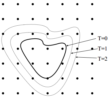
Solving the adjoint can then be described as propagating rays through the medium and then backtracing the residual value back through the volume.

The discrete adjoint

If we instead use a discretized version of the eikonal equation, our Lagrangian becomes

\mathcal{L} = \underset{i \in \text{meas}}{\sum} \left(\Phi_i - \hat{\Phi}_i \right)^2 \\ - \underset{i \in \Omega}{\sum} \lambda_i \left((\mathbf{D}_x\Phi_i)^2 + (\mathbf{D}_y \Phi_i)^2 - \eta^2_i \right)

We differentiate with respect to each \(\Phi_i\) and \(\lambda_i\) to get a linear system

The discrete adjoint

\mathcal{L} = \underset{i \in \text{meas}}{\sum} \left(\Phi_i - \hat{\Phi}_i \right)^2 \\ - \underset{i \in \Omega}{\sum} \lambda_i \left((\mathbf{D}_x\Phi_i)^2 + (\mathbf{D}_y \Phi_i)^2 - \eta^2_i \right)
\begin{bmatrix} 0 \\ \Phi - \hat{\Phi} \end{bmatrix} - \begin{bmatrix} d\Phi_0^T \\ d\Phi_1^T \\ \cdots \\ d\Phi_i^T \end{bmatrix} \lambda = 0

\(\lambda\) here acts exactly in the same way as the continuous version

Concluding Thoughts

  • Adjoint State Method is Lagrange Multipliers in disguise
  • The broad theory for the adjoint state method can be used to tackle inverse problems
  • The adjoint state in the eikonal case amounts to backtracing rays back through the volume to deposit the gradient value

References and Links