Reinforcement Learning
Learning Objectives
-
Understand the concept of exploration, exploitation, regret
-
Describe the relationships and differences between:
-
Markov Decision Processes (MDP) vs Reinforcement Learning (RL)
-
Model-based vs Model-free RL
-
Temporal-Difference Value Learning (TD Value Learning) vs Q-Learning
-
Passive vs Active RL
-
Off-policy vs On-policy Learning
-
Exploration vs Exploitation
-
-
Describe and implement:
-
Temporal difference learning
-
Q-Learning
-
\(\epsilon\)-Greedy algorithm
-
Approximate Q-learning (Feature-based)
-
-
Derive weight update for Approximate Q-learning
Definitions
Before diving into the details, let’s look at a high-level overview outlining vocabulary terms
we’ll see
come up and contrasting different methods.
It would also be useful to revisit this section after you’ve reviewed the specific RL algorithms and
have a more
concrete view of things.
First off, our distinction between MDPs and RL in this class might be a little misleading - MDPs refer to
the way we
formulate the environment, and we use RL methods to derive useful information (like state values or optimal
policies)
about the MDP. The algorithms seen before (value and policy iteration) can still be considered RL,
they’re just
offline (so some might consider them more "solving" than "learning").
Online learning: Learn by taking actions and observing outcomes in some
environment.
Offline learning: Learn by the environment dynamics information alone, without needing to
act in the
environment.
\(\Rightarrow\) Requires access to the MDP’s transition and reward
functions.
Within online learning, we can also have
Passive learning: the policy \(\pi\) we follow as we
explore is
fixed, and we passively follow it. Generally the goal with passive learning is just to evaluate states or
our
policy.
Active learning: the policy we follow changes over time.
Another categorization within online learning is model-based vs. model-free learning.
Model-based learning: we first try to model the environment (usually by estimating the
transition and
reward functions).
\(\Rightarrow\) This can be accompanied by offline learning
methods.
Model-free learning: we learn evaluations/policies without trying to model the
environment.
A third and final categorization is on-policy vs. off-policy learning.
On-policy learning: the policy we’re evaluating/improving is the current policy
we’re
following.
Off-policy learning: the policy we’re improving/evaluating is a different policy than
the one
we follow (e.g., the optimal policy \(\pi^*\)).
This can be summarized in the slide below, though note that on- vs. off-policy is not depicted
here.

While there are tons of online learning algorithms out there, the two we focus on in this class are temporal difference (TD) learning and Q-learning.
TD Learning
TD learning estimates the utility of states from action-outcome information. Say we have some initial estimate of the utility of a state \(s\), notated as \(V_0(s)\), and we observe a sample \((s, a, s', R(s, a, s'))\) (note that we do not have access to the complete reward function \(R\), only specific values gleaned from experience). How should we go about updating our utility estimate to take into account this new information? Consider two extremes:
-
We only account for the new observation. Then our new estimate \(V_1(s)\) will be \(R(s, a, s') + \gamma V_0(s')\). This utilizes the new information, but is not very accurate. The sample could have been of a transition that occurs only 1 percent of the time when taking action \(a\), and we would then be basing our entire estimate on a 1 percent corner case.
-
We disregard the new observation. Then our new estimate \(V_1(s)\) will be \(V_0(s)\). We won’t be vulnerable to skewing by rare transitions as in the first case, but our estimate will also not get any more accurate no matter how much data we throw at it.
As you might expect, the better strategy is to incorporate both the utility estimate from prior experiences as well as the new sample into an updated utility. This notion can be expressed mathematically as a weighted average of the two values: \(V_{i + 1}(s) = (1 - \alpha)V_i(s) + \alpha (R(s, a, s') + \gamma V_i(s'))\). (Question: can you express the two cases above with this formula?). \(\alpha\) is often called the "learning rate". As its value increases, we give more weight to new observations, and vice versa.
Where does the term "temporal difference" come from? With a little bit of rearranging, the TD update rule becomes \(V_{i + 1}(s) = V_i(s) + \alpha ((R(s, a, s') + \gamma V_i(s')) - V_i(s))\). This can be interpreted as updating the utility estimate using the difference between states, scaled by \(\alpha\).
If \(\alpha\) is a constant, the value estimates themselves will not
necessarily
converge to optimal although a running average of the estimates for each state will (why?). We can
guarantee
a
convergence to the optimal values however by decreasing \(\alpha\)
appropriately over
time.
Example
We have a layout of 4 states: Kitchen, Bedroom, Living Room, and Laundry Room. We want to use TD Learning to compute the values of these states.

Now that we are in the world of online learning (i.e. we do not have access to a reward function or transition function as we did in MDPs), the only way we can know what rewards result from taking what actions from specific states is by acting out in our environment.
Suppose we observe the following \((s,a,s', R(s,a,s'))\) transitions and rewards:
-
\((Kitchen, MOVE, Laundry, 2)\)
-
\((LivingRoom, MOVE, Kitchen, 6)\)
-
\((Bedroom, PLAY, LivingRoom, 1)\)
-
\((Kitchen, MOVE, Laundry, 2)\)
-
\((LivingRoom, PLAY, Laundry, 4)\)
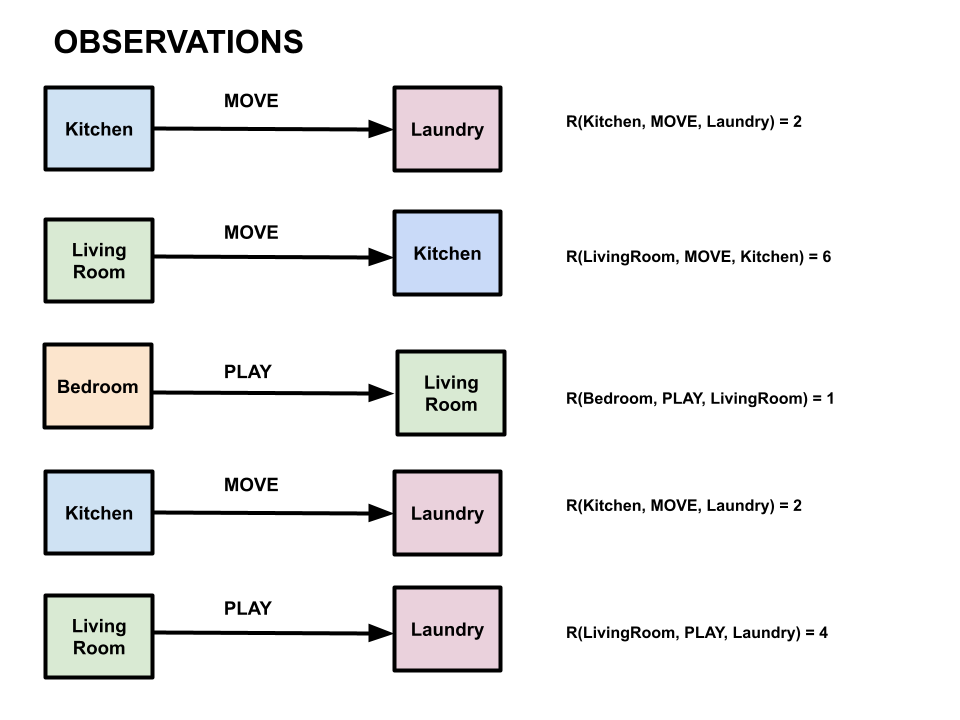
Note that the \(R(s,a,s')\) in this notation refers to observed reward, not a reward value computed from a reward function (because we don’t have access to the reward function).
Let our discount factor \(\gamma=1\) and our learning rate \(\alpha=0.6\)
Substituting these into our formulation for a single update of TD-learning, we have \[\begin{align*} V^\pi(s) &\leftarrow (1 - \alpha)V^\pi(s) + \alpha[R(s, \pi(s), s') + \gamma V^\pi(s')] \\ & \leftarrow (1 - 0.6)V^\pi(s) + 0.6 [R(s, \pi(s), s') + 1 V^\pi(s')] \\ & \leftarrow 0.4 V^\pi(s) + 0.6 [R(s, \pi(s), s') + V^\pi(s')] \end{align*}\]
What are the learned values for each state from TD learning after all five observations?
Using the table below, we will keep track of the learned values for each state after the five observations. We will map each state to a value, and initialize the value of each state to 0. The table below has the final values with the step by step calculations below.
| Transitions | Kitchen | LivingRoom | Bedroom | Laundry |
|---|---|---|---|---|
| (initial) | 0 | 0 | 0 | 0 |
| (Kitchen, MOVE, Laundry, 2) | 1.2 | 0 | 0 | 0 |
| (LivingRoom, MOVE, Kitchen, 6) | 1.2 | 4.32 | 0 | 0 |
| (Bedroom, PLAY, LivingRoom, 1) | 1.2 | 4.32 | 3.19 | 0 |
| (Kitchen, MOVE, Laundry, 2) | 1.68 | 4.32 | 3.19 | 0 |
| (LivingRoom, PLAY, Laundry, 4) | 1.68 | 4.13 | 3.19 | 0 |
We will update the values after observing each transition.
After our first observation, \((Kitchen, MOVE, Laundry, 2)\), we update \(V^\pi(Kitchen)\) \[\begin{align*} V^\pi(Kitchen) & \leftarrow 0.4 V^\pi(Kitchen) + 0.6 [R(Kitchen, MOVE, Laundry) + V^\pi(Laundry)] \\ & \leftarrow 0.4 (0) + 0.6 [2 + 0] \\ & \leftarrow 1.2 \end{align*}\]
Similarly, after observing \((LivingRoom, MOVE, Kitchen, 6)\), we update \(V^\pi(LivingRoom)\) \[\begin{align*} V^\pi(LivingRoom) & \leftarrow 0.4 V^\pi(LivingRoom) + 0.6 [R(LivingRoom, MOVE, Kitchen) + V^\pi(Kitchen)] \\ & \leftarrow 0.4 (0) + 0.6 [6 + 1.2] \\ & \leftarrow 4.32 \end{align*}\]
Now, we observe \((Bedroom, PLAY, LivingRoom, 1)\). We update \(V^\pi(Bedroom)\) \[\begin{align*} V^\pi(Bedroom) & \leftarrow 0.4 V^\pi(Bedroom) + 0.6 [R(Bedroom, PLAY, LivingRoom) + V^\pi(LivingRoom)] \\ & \leftarrow 0.4 (0) + 0.6 [1 + 4.32] \\ & \leftarrow 3.19 \end{align*}\]
Next, we observe \((Kitchen, MOVE, Laundry, 2)\) again, and we update \(V^\pi(Kitchen)\). \[\begin{align*} V^\pi(Kitchen) & \leftarrow 0.4 V^\pi(Kitchen) + 0.6 [R(Kitchen, MOVE, Laundry) + V^\pi(Laundry)] \\ & \leftarrow 0.4 (1.2) + 0.6 [2 + 0] \\ & \leftarrow 1.68 \end{align*}\]
Finally, we observe \((LivingRoom, PLAY, Laundry, 4)\), and we update \(V^\pi(LivingRoom)\) \[\begin{align*} V^\pi(LivingRoom) & \leftarrow 0.4 V^\pi(LivingRoom) + 0.6 [R(LivingRoom, PLAY, Laundry) + V^\pi(Laundry)] \\ & \leftarrow 0.4 (4.32) + 0.6 [4 + 0] \\ & \leftarrow 4.13 \end{align*}\]
Q-Learning
TD-learning has a weakness in that we can use it to estimate the utilities of states under a given policy, but given that information, we cannot directly extract an optimal policy since we don’t have a model of the transition probabilities or rewards. Q-learning fixes this by instead modeling Q-values, the expected utility of taking a particular action at a particular state. Recall that the optimal policy is characterized in terms of Q-values by \[\pi^*(s) = \text{argmax}_a Q(s, a)\ \forall s\] The update rule for Q-learning takes a weighted average between the previous Q-value estimate and the utility estimated from the observed transition: \[Q_{i + 1}(s, a) = (1 - \alpha)Q_i(s, a) + \alpha (R(s, a, s') + \gamma V_i(s'))\] Where we use the utility/Q-value relationship \(V(s) = max_a Q(s, a)\) to rewrite this as \[Q_{i + 1}(s, a) = (1 - \alpha)Q_i(s, a) + \alpha (R(s, a, s') + \gamma max_{a'}Q(s', a'))\] We can also rewrite this in a difference form (similar to gradient descent): \[Q_{i + 1}(s, a) = Q_i(s, a) + \alpha (R(s, a, s') + \gamma max_{a'}Q(s', a') - Q(s, a))\]
Example
Continuing with the example we set up in the previous section, we now want to perform Q-learning so that we can find the values of each (state, action) pair. Let Q(s,a)=0 initially for all Q-states (s,a),. Let \(\alpha=0.6\) and \(\gamma = 1\).
We use the following Q-value update rule to find what the new value should be (note what is inside of the brackets may also be referred to as sample in the slides): \[Q(s, a) = (1 - \alpha)Q(s, a) + \alpha [R(s, a, s') + \gamma max_{a'}Q(s', a')]\]
Updating this with the values we already know, we get: \[Q(s, a) = (0.4)Q(s, a) + 0.6 [R(s, a, s') + max_{a'}Q(s', a')]\]
The final results are as follows with the calculations shown below the table:
| Transitions | (K, MOVE) | (LR, MOVE) | (B, PLAY) | (LR, PLAY) |
|---|---|---|---|---|
| (initial) | 0 | 0 | 0 | 0 |
| (K, MOVE, L, 2) | 1.2 | 0 | 0 | 0 |
| (LR, MOVE, K, 6) | 1.2 | 4.32 | 0 | 0 |
| (B, PLAY, LR, 1) | 1.2 | 4.32 | 3.19 | 0 |
| (K, MOVE, L, 2) | 1.68 | 4.32 | 3.19 | 0 |
| (LR, PLAY, L, 4) | 1.68 | 4.32 | 3.19 | 2.4 |
In the first observation, we see \((Kitchen, MOVE, Laundry, 2)\) so we update the Q-value for (Kitchen, MOVE). \[\begin{align*} Q(K, MOVE) &= 0.4 Q(K, MOVE) + 0.6 [R(K, MOVE, L) + max_{a'}Q(L, a')] \\ & = 0.4 (0) + 0.6 [2 + 0] \\ & = 1.2 \end{align*}\]
Next, we see \((LivingRoom, MOVE, Kitchen, 6)\) so we update the Q-value for (LivingRoom, MOVE). \[\begin{align*} Q(LR, MOVE) &= 0.4 Q(LR, MOVE) + 0.6 [R(LR, MOVE, K) + max_{a'}Q(K, a')] \\ & = 0.4 (0) + 0.6 [6 + 1.2] \\ & = 4.32 \end{align*}\]
Next, we see \((Bedroom, PLAY, LivingRoom, 1)\) so we update the Q-value for (Bedroom, PLAY). \[\begin{align*} Q(B, PLAY) &= 0.4 Q(B, PLAY) + 0.6 [R(B, PLAY, LR) + max_{a'}Q(LR, a')] \\ & = 0.4 (0) + 0.6 [1 + 4.32] \\ & = 3.19 \end{align*}\]
Next, we see \((Kitchen, MOVE, Laundry, 2)\) again so we update the Q-value for (Kitchen, MOVE). \[\begin{align*} Q(K, MOVE) &= 0.4 Q(K, MOVE) + 0.6 [R(K, MOVE, L) + max_{a'}Q(L, a')] \\ & = 0.4 (1.2) + 0.6 [2 + 0] \\ & = 1.68 \end{align*}\]
Next, we see \((LivingRoom, PLAY, Laundry, 4)\) so we update the Q-value for (LivingRoom, PLAY). \[\begin{align*} Q(LR, PLAY) &= 0.4 Q(LR, PLAY) + 0.6 [R(LR, PLAY, L) + max_{a'}Q(L, a')] \\ & = 0.4 (0) + 0.6 [4 + 0] \\ & = 2.4 \end{align*}\]
Count Exploration Q-Learning
Another type of Q-learning that we can implement, other than epsilon-greedy Q-learning, is Count Exploration Q-learning. In this type of Q-learning, we augment our Q values with an extra term as follows, where u represents the original Q-value, k is a hyperparameter and n is the number of times we have "visited" the (state, action) pair.
\[f(u, n) = u + \frac{k}{n+1}\]
We can utilize our f-function to construct our new Q-value update rule.
Here is the original Q-update rule for reference:\[Q(s,a) = Q(s,a) + \alpha (r + \gamma max_{a'}Q(s', a') - Q(s, a))\]
We now instead use this modified Q-update rule for count-exploration Q-learning:\[Q'(s,a) = Q'(s,a) + \alpha (r + \gamma max_{a'}f(Q'(s', a'), N(s', a')) - Q'(s, a))\]
This incentivizes the agent to explore states which it has seen less or not seen at all. This can outperform epsilon greedy search in some scenarios.
For example, if a long sequence of actions initially has low rewards, but gives a very large reward at the end, epsilon greedy may fail to explore this sequence of actions as it would happen randomly with low probability and the initial Q values would be too low for it to be explored otherwise. With the count exploration function, however, the agent would be incentivized to eventually explore these unseen states before (assuming k is large enough). One disadvantage is the necessity of choosing the extra hyperparameter k.
There are many more interesting examples of exploration functions that are out of scope for this class.
Exploration vs Exploitation
A classic ongoing question in RL is how to trade off exploration vs. exploitation - that is, how to strike the right balance between exploring new/fewer-seen states and exploiting our current knowledge by taking actions we know are good.
One possible answer to this question is to use augment whatever online algorithm we’ve chosen with \(\epsilon\)-greedy exploration. Using an \(\epsilon\)-greedy strategy means we take a random action with probability \(\epsilon\), and follow our policy with probability \(1 - \epsilon\).
A related concept to explore/exploit is regret, the difference between the sum of rewards we actually received at some point in our learning and the sum of rewards had we followed an optimal policy. As you might guess, more exploration might accumulate more regret early on, but helps ensure that we learn the optimal policy in the long run.
Approximate Q-Methods
All the algorithms we’ve seen so far work well enough, but are only really guaranteed to converge if all states are visited enough times. What if our state space is really big, like infinitely big? Approximate learning methods aim to get around this by using features of states and learning a function to approximate state values based on the values of those features. In this class we look at approximate Q-learning.
Approximate Q-Learning
One approximate solution is to generalize states by mapping them to sets of features and calculating
Q-values based
on those features instead of states.
Features are mappings from states to some real number, sometimes normalized to be between 0 and 1. For
Pacman, some
example features might be the ratio of remaining food pallets and total pallets, or minimum distance from
ghosts.
A simple way to combine all features to generate approximate Q-values is through a linear value
function/dot product
between weights and feature values: \[Q_w(s, a) = w_1f_1(s, a) + w_2f_2(s,a)
+...+w_nf_n(s,a)\] where weight \(w_i\) can be seen as how
valuable our
agent thinks feature \(f_i\) is. Recall that you had to come up with
these
weights
yourself when creating evaluation functions on P1. Now, we’re going to have the agent learn the best
weights
through experience. Then, during the learning stage instead of updating q values, we update the weights
instead.
What is our ideal set of weights, given a newly observed sample? One that minimizes the error between our
estimate and
the utility predicted by that sample. In math: \[w^*_1, \ldots, w^*_n =
\text{argmin}_{w_1,
\ldots, w_n}Error(sample, Q_w(s, a))\] Where \(Error(x, y) =
\frac{1}{2}(x -
y)^2\), the classic least-squares error function. We do this by moving each weight opposite the
direction of
increasing error, using the following weight update equation: \[w_i \leftarrow
w_i -
\alpha\frac{\partial Error}{\partial w_i}\]
For some intuition on this, think about how you would, standing at some point on a hill (say in a thickly
wooded
forest so you have no other cues) and observing the slope, determine which direction to go to descend or
ascend.
Now, \(f_i(s, a) = \frac{\partial Q_w(s, a)}{\partial w_i}\) and \(-[sample - Q_w(s, a)] = \frac{\partial Error}{\partial Q_w(s, a)}\).
Hence, multiplying the two gives \((\frac{\partial Error}{\partial Q_w(s,
a)})(\frac{\partial
Q_w(s,
a)}{\partial w_i}) = \frac{\partial Error}{\partial w_i}\) by the chain rule.
Substituting in
this
expression
and recalling that \(sample = R(s, a, s') + \gamma \max_{a'} Q(s', a')\),
we derive
the weight update rule for linear approximate Q functions: \[w_i \leftarrow w_i
+
\alpha
[R(s, a, s') + \gamma \max_{a'} Q(s', a') - Q(s, a)]f_i(s, a)\]
Example
Prince is too lazy to keep track of all of the possible (state, action) pairs so he decides to use
Approximate
Q-learning (because he is smart and savvy like that). He ends up using two features \(f_1\) and \(f_2\)
that
have
corresponding weights \(w_1\) and \(w_2\).
His approximation function is as follows: \[Q_w(s,a)
=
w_1f_1(s,a) + w_2f_2(s,a)\]
Assume that:
- \(f_1(Bedroom, PLAY) = 3\) and \(w_1 = 1\)
- \(f_2(Bedroom, PLAY) = 1\) and \(w_2 = 2\)
- \(\gamma = 0.5\), \(\alpha = 0.5\)
Based on the features and weights described above, we can calculate the approximate Q-value for (Bedroom,
PLAY).
\[Q_w\text{(Bedroom, PLAY)} = 1(3) + 2(1) = 5\] If we were to observe the transition and reward
\((Bedroom,
PLAY,
LivingRoom, 2)\), we can now calculate the \(Q_{sample}\) for (Bedroom, PLAY). We can assume for the sake
of
the
example that \(max_{a'}Q_w(LivingRoom, a’) = 8\).
Using the equation: \(Q_{sample}(s,a) = R +
\gamma(max_{a'}Q_w(s',a')\)), we get: \[Q_{sample}(Bedroom, PLAY) = 2 + 0.5(8) = 6\] Now that we have
made
an
observation and calculated the Q-values, we can update the weights!
\[w_1 = 1 + 0.5[6 - 5](3) = 2.5\]
\[w_2 = 2 + 0.5[6 - 5](1) = 2.5\]
These are our new weights that we can then use in the calculation of future observed states.