Markov Decision Processes
Learning Objectives
-
Describe the definition of Markov Decision Process
-
Compute utility of a reward sequence given discount factor
-
Define policy and optimal policy of an MDP
-
Define state-value and (true) state value of an MDP
-
Define Q-value and (true) Q value of an MDP
-
Derive optimal policy from (true) state value or (true) Q-values
-
Write Bellman Equation for state-value and Q-value for optimal policy and a given policy
-
Describe and implement value iteration algorithm (through Bellman update) for solving MDPs
-
Describe and implement policy iteration algorithm (through policy evaluation and policy improvement) for solving MDPs
-
Understand convergence for value iteration and policy iteration
Defining MDPs
Formulation
A Markov Decision Process (MDP) is defined by:
-
A set of states \(S\). For pacman this could be grid positions.
-
A set of actions \(A\). For pacman, this would be North, South, East, and West.
-
A transition function \(T(s, a, s')\) which represents the probability of being in state \(s'\) after taking action \(a\) from state \(s\).
-
A reward function \(R(s, a, s')\) which represents the reward received from being in state \(s\), taking action \(a\), and ending up in state \(s'\).
-
A start state \(s_0\in S\)
-
Potentially one or more terminal states
Markov Property
The Markov property says that given the present state, the previous and future states are all conditionally independent.
In the
context of MDPs, this means that actions depend only on the current state. That is to say, the following two
expressions are equivalent for MDPs:
\(P(S_{t+1}=s_{t+1}|A_t=a_t, s_t=s_t,
A_{t-1}=a_{t-1}, S_{t-1}=s_{t-1}...A_0=a_0,
S_0=s_0)\)
\(P(S_{t+1}=s_{t+1}|A_t=a_t, s_t=s_t)\)
Policies
A policy, \(\pi\), represents our plan. More formally, \(\pi\) is a function that maps states to actions (\(\pi: S
\rightarrow A\)). For each state \(s\in S\), \(\pi(s)\) will return the corresponding action from our plan.
An optimal policy is one that would maximize our expected utility if followed.
Exercise: How is this different than what expectimax does (hint: does expectimax tell you what to do for every state)?
Discounting
The idea of discounting stems from the common idea that a reward now is better than the same reward later on. Therefore, according to this philosophy, we want to weight each value of a state by some factor \(\gamma \in [0, 1]\). If we do not restrict \(\gamma\) to this range, the game could last forever with the reward being infinite.
More concretely, the reward is worth \(\gamma^0*R\) now, and \(\gamma^1*R\) after one step and \(\gamma^2R\) after two, and so on. This is to ensure that we prioritize rewards now rather than later on in our path to the goal. A \(\gamma\) closer to 0 will mean that we have a smaller horizon and care more about immediate rewards and actions while a \(\gamma\) closer to 1 will weigh later rewards almost equally to immediate rewards.
Solving MDPs
For now, we are assuming we have access to all dynamics information about some particular MDP, i.e., the
transition
(\(T \text{ or } P\)) and reward (\(R\)) functions. If
this is
the case, we can directly solve for the optimal value function (what is the expected utility I get from
being in some
state \(s\), assuming I act optimally), which helps us get the optimal
policy in this
environment. Two such algorithms are value iteration and policy
iteration.
The methods described here are offline learning methods, as we don’t have to actually
take
actions in the environment to derive a value function/policy. In Reinforcement Learning, we’ll get to
online
learning methods.
Throughout the rest of this note, we will refer to the same example described below:
Example
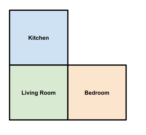
Prince the dog is roaming the house in search of food, toys or anything to play with he can get his paws
on.
Prince’s house is shown in the picture below. From each room in the house he can decide to play or
move from
room to room without playing. Moving gives him no reward but playing and ending up in certain rooms can
affect how
much reward Prince get. A positive reward indicates that Prince received a treat and a negative reward means
that he
was in trouble :(. Below the house map, you can see the rewards and transitions for each possible state and
action.
Help Prince find out what his expected values are depending on the room he is in as well as what is the best
action to
take from each state!

Value Iteration
Recall that a state’s value, denoted \(V(s)\) is the expected utility for starting out in that state and acting optimally. We also use the term Q-value, denoted \(Q(s, a)\), which is the expected utility of starting out in state \(s\), taking action \(a\), and then acting optimally.
Intuitively, the optimal Q-value for a state can be defined as: \[Q^*(s, a) = \sum_{s'\in S}T(s, a, s')(R(s, a, s') + \gamma V^*(s'))\] where \(V^*\) is the optimal value, and can be defined as \[V^*(s) = \max\limits_{a}Q(s, a)\]
In English, we can explain the Q-value as weighted sum over all possible reachable states from \(s\) by doing action \(a\) of the reward for landing in state \(s'\) plus the value of \(s'\) discounted by \(\gamma\). The weights in this case would be the probability of getting to \(s'\), so we’d weight more likely states higher. The optimal value of a state is just the max Q-value over all actions possible for that state. One common algorithm to find the values of each of these states is value iteration.
Algorithm
Value iteration can be summarized with the following Bellman update equation: \[V(s) = \max\limits_{a}\sum_{s'\in S}T(s, a, s')(R(s, a, s') + \gamma V(s'))\]
Each update can be thought of as computing one ply of the expectimax search tree. The actual algorithm is as follows:
-
Initialize the values of all states to be 0
-
Apply the update rule: \[V_{k+1}(s) = \max\limits_{a}\sum_{s'\in S}T(s, a, s')(R(s, a, s') + \gamma V_k(s'))\]to all states
-
Repeat step 2 until convergence
The complexity of a single iteration of value iteration is \(O(|S|^2|A|)\) because for every state, we must go through all of the actions, and for each action, go through all of the other possible states the agent can get to (which in the worst case will be \(|S|\)).
This can also be thought of in terms of Q-values, giving us Q-value iteration. This follows the same steps as above except initializing all Q-values to zero and using this update rule: \[Q_{k+1}(s, a) = \sum_{s'\in S}T(s, a, s')(R(s, a, s') + \gamma \max\limits_{a'}Q_k(s', a'))\]
Exercise: Try to convince yourself that these two methods are essentially doing the same thing (hint: what is the definition of a Q-value?).
At the end of Q-value iteration, you can convert to values by: \[V^*(s) = \max\limits_{a}Q^*(s, a)\]
Convergence Criteria
We are told in theory that value iteration will converge to the unique optimal values for each
state.
Here is a quick sketch of the proof: by cases:
Case 1: If the expectimax search tree is finite with \(M\)
levels,
then value iteration will converge, and \(V_M\) (the values at the Mth level) will hold the optimal values
Case 2 (\(\gamma < 1\)): For any state \(s\), \(V_k(s), V_{k+1}(s)\) can be viewed as
depth
\(k+1\) expectimax results in nearly identical search trees. However, the
bottom most
layer for \(V_k\) will be zero but for \(V_{k+1}\)
will be rewards. The extrema for \(V_{k+1}\) are \(R_{min}\) and \(R_{max}\). So that means
that the
difference between the bottom most layers is \(\gamma^k \max |R|\) but
since \(\gamma < 1\) the difference will get smaller and smaller each
layer and eventually
converge.
Example
We will now run value iteration on our Prince’s House Example described above with a \(\gamma\) of 0.8. Below is the table of the values we get from running value iteration with the math corresponding to each cell shown below the table.
| Iteration | Kitchen | Living Room | Bedroom |
|---|---|---|---|
| \(V_0\) | 0 | 0 | 0 |
| \(V_1\) | 1 | 0 | 0 |
| \(V_2\) | 1 | 0.475 | 0 |
| \(V_3\) | 1 | 0.475 | 0 |
\(\mathbf{V_0}\): We initialize all values to 0.
\(\mathbf{V_1}\):
-
\(V_1(\)Kitchen\() = max(1(1+0.8(0)), 1(0+0.8(0))) = max(1, 0) = 1\)
-
\(V_1(\)Living Room\() = max(0.75(-0.5+0.8(0)) + 0.25(1+0.8(0)), 1(0+0.8(0))) = max(-0.125, 0) = 0\)
-
\(V_1(\)Bedroom\() = 0\) because it is a terminal state where no actions can be done.
\(\mathbf{V_2}\):
-
\(V_2(\)Kitchen\() = max(1(1+0.8(0)), 1(0+0.8(0))) = max(1, 0) = 1\)
-
\(V_2(\)Living Room\() = max(0.75(-0.5+0.8(1)) + 0.25(1+0.8(0)), 1(0+0.8(0))) = max(0.475, 0) = 0.475\)
-
\(V_2(\)Bedroom\() = 0\) because it is a terminal state where no actions can be done.
\(\mathbf{V_3}\):
-
\(V_3(\)Kitchen\() = max(1(1+0.8(0)), 1(0+0.8(0.475))) = max(1, 0.38) = 1\)
-
\(V_3(\)Living Room\() = max(0.75(-0.5+0.8(1)) + 0.25(1+0.8(0)), 1(0+0.8(0.475))) = max(0.475, 0.38) = 0.475\)
-
\(V_3(\)Bedroom\() = 0\) because it is a terminal state where no actions can be done.
The values have converged so we stop value iteration and return the optimal values that we got in the most recent iteration.
Policy Extraction
Value iteration is an algorithm to get the optimal values for all states in the agent’s world.
However, it does
not tell the agent what action to take in a given state, we would need a policy for that.
For any given set of values \(V\), we can find the corresponding policy
(\(\pi_V\)) using policy extraction, defined as follows: \[\pi_V(s) = argmax_a \sum_{s'\in S}T(s, a, s')(R(s, a, s') + \gamma V(s'))\]
We choose
the action that yields the highest value.
Policy Iteration
Another method of solving MDP’s is policy iteration, which consists of policy evaluation and policy improvement.
Policy Evaluation
Policy evaluation consists of calculating the values for some fixed policy, \(\pi_i\), until convergence. The values, \(V^{\pi_i}(s)\), represent the expected total discounted rewards starting in
state s and
following \(\pi_i\).
The recursive relationship of the utility of a state under a fixed policy can be expressed as follows. This is also known as one-step look ahead. \[V^{\pi_i}(s) = \sum_{s'} T(s, \pi_i(s), s')[R(s, \pi_i(s), s') + \gamma V^{\pi_i}(s')]\]
In order to actually calculate the values for a fixed policy, there are two methods we can use. First, we can iterate over the recursive equation above and update the values until convergence. This will give us the following update rule: \[V_{k+1}^{\pi_i}(s) = \sum_{s'} T(s, \pi_i(s), s')[R(s, \pi_i(s), s') + \gamma V_k^{\pi_i}(s')]\]
We observe that by using a fixed policy, this eliminates an additional loop over all possible actions which
brings
the time complexity for each iteration down to \(O(S^2)\).
Another (optional) method to solve for the values is to solve them as a system of equations. By eliminating
the \(\max_{a}\), the equations are now just a linear system of equations
which can be
written in vector form and solved for.
Policy Improvement
After running policy evaluation using our fixed policy, \(\pi\), we now want to improve upon \(\pi\) by running one ply of the Bellman equations. \[\pi_{i+1}(s) = argmax_a \sum_{s'} T(s, a, s') [R(s, a, s') + \gamma V^{\pi_i}(s')]\]
We will then run policy evaluation on this new policy and keep repeating this process until the policy converges.
Example
We now want to help Prince find the optimal policy for him to maximize his treat intake so we want to run policy iteration. We will start with the base policy that Prince moves whether he is in the Kitchen or the Living Room and with a discount factor of 0.8. The table below shows all of the values and polices we get with the calculations below the table.
| Iteration | Kitchen | Living Room | Bedroom |
|---|---|---|---|
| \(\pi_0\) | Move | Move | N/A |
| \(V_0^{\pi_0}\) | 0 | 0 | 0 |
| \(V_1^{\pi_0}\) | 0 | 0 | 0 |
| \(\pi_1\) | Play | Move | N/A |
| \(V_0^{\pi_1}\) | 0 | 0 | 0 |
| \(V_1^{\pi_1}\) | 1 | 0 | 0 |
| \(V_2^{\pi_1}\) | 1 | 0 | 0 |
| \(\pi_2\) | Play | Play | N/A |
| \(V_0^{\pi_2}\) | 0 | 0 | 0 |
| \(V_1^{\pi_2}\) | 1 | -0.125 | 0 |
| \(V_2^{\pi_2}\) | 1 | 0.475 | 0 |
| \(V_3^{\pi_2}\) | 1 | 0.475 | 0 |
| \(\pi_3\) | Play | Play | N/A |
POLICY 0 \(\pi_0\)
Policy evaluation:
-
\(V_0\): all values initialized to 0
-
\(V_1\):
-
\(V_1(\)Kitchen\() = 1(0 + 0.8(0)) = 0\)
-
\(V_1(\)Living Room\() = 1(0+0.8(0)) = 0\)
-
Values converged so now we must extract the new policy.
Policy Improvement: Assume the first value is for Play and the second is for Move in the argmax
-
\(\pi_1(\)Kitchen\() = argmax(1(1+0.8(0)), 1(0+0.8(0))) = argmax(1, 0)\) = Play
-
\(\pi_1(\)Living Room\() = argmax(0.75(-0.5+0.8(0)) + 0.25(1+0.8(0)), 1(0+0.8(0))) = argmax(-0.125, 0)\) = Move
POLICY 1 \(\pi_1\)
Policy evaluation:
-
\(V_0\): all values initialized to 0 (cold start)
-
\(V_1\):
-
\(V_1(\)Kitchen\() = 1(1 + 0.8(0)) = 1\)
-
\(V_1(\)Living Room\() = 1(0+0.8(0)) = 0\)
-
-
\(V_2\):
-
\(V_2(\)Kitchen\() = 1(1 + 0.8(0)) = 1\)
-
\(V_2(\)Living Room\() = 1(0+0.8(0)) = 0\)
-
Values converged so now we must extract the new policy.
Policy Improvement: Assume the first value is for Play and the second is for Move in the argmax
-
\(\pi_2(\)Kitchen\() = argmax(1(1+0.8(0)), 1(0+0.8(0) = argmax(1, 0)\) = Play
-
\(\pi_2(\)Living Room\() = argmax(0.75(-0.5+0.8(1)) + 0.25(1+0.8(0)), 1(0+0.8(0))) = argmax(0.475, 0)\) = Play
POLICY 2 \(\pi_2\)
Policy evaluation:
-
\(V_0\): all values initialized to 0 (cold start)
-
\(V_1\):
-
\(V_1(\)Kitchen\() = 1(1 + 0.8(0)) = 1\)
-
\(V_1(\)Living Room\() = 0.75(-0.5+0.8(0)) + 0.25(1+0.8(0)) = -0.125\)
-
-
\(V_2\):
-
\(V_2(\)Kitchen\() = 1(1 + 0.8(0)) = 1\)
-
\(V_2(\)Living Room\() = 0.75(-0.5+0.8(1)) + 0.25(1+0.8(0)) = 0.475\)
-
-
\(V_2\):
-
\(V_2(\)Kitchen\() = 1(1 + 0.8(0)) = 1\)
-
\(V_2(\)Living Room\() = 0.75(-0.5+0.8(1)) + 0.25(1+0.8(0)) = 0.475\)
-
Values converged so now we must extract the new policy.
Policy Improvement: Assume the first value is for Play and the second is for Move in the argmax
-
\(\pi_3(\)Kitchen\() = argmax(1(1+0.8(0)), 1(0+0.8(0.475)) = argmax(1, 0.38)\) = Play
-
\(\pi_3(\)Living Room\() = argmax(0.75(-0.5+0.8(1)) + 0.25(1+0.8(0)), 1(0+0.8(0.475))) = argmax(0.475, 0.38)\) = Play
The policy has now converged so we can tell Prince that if he is always playing he will maximize his treat intake and he is expected to get a treat in both rooms! Also take note that policy iteration and value iteration converged to the same values. If we took the argmax based on the values we got from value iteration we would have gotten the same optimal policy that we just found.
Summary
Both value iteration and policy iteration are dynamic programs that compute optimal values for solving MDPs. Value iteration doesn’t explicitly track a policy but we implicitly recompute it by taking a max over the actions. On the other hand, policy iteration does keep track of a policy and we perform multiple passes to improve upon it. By considering only one action per state, each iteration takes less time. However, unlike value iteration, we perform several passes of policy evaluation and policy improvement.