Classical Planning

Learning Objectives

Compare and contrast classical planning methods with planning via search or propositional logic
Execute linear planning algorithms on real-world problems
Describe and identify the difference between linear and nonlinear planning algorithms
Identify properties of a given planning algorithm, namely whether it is sound, complete, and optimal
Discuss how GraphPlan differs from searching in a state-space graph representation
Identify termination conditions from a GraphPlan planning graph
Implement and execute real-world planning problems using GraphPlan

Classical Planning Representation

In classical planning, we aren't constrained to symbols that only take on true or false values, as we were in propositional logic. Instead, we introduce objects that can represent things in our environment. We let predicates, also called propositions, be true or false functions over the objects.

A state is a conjunction of predicates. Similarly, our goal will also be a conjunction of predicates.

Operators change the state by adding or deleting predicates. An operator is defined by preconditions and effects. The preconditions specify all the predicates that need to be true in our current state in order for us to take this action. The effects are the predicates that we need to add or delete from our current state after we take this action. Notice that we do not explicitly represent time in classical planning, unlike the successor-state axioms in propositional logic. Important: there is a difference between deleting a predicate and adding its negation. We can require as a precondition the negation of a predicate, but we can’t require the absence of a predicate.

We can use variables in operators to represent that one of multiple objects of the same type could be operated on.

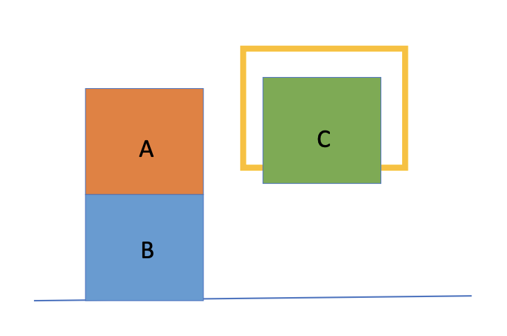
For example, consider the image above - we have blocks A, B, and C and a hand that can pick up any of the blocks. One example of a predicate might be On-Table(B) that specifies whether object B is on the table or not. In order to represent the above state, we would need objects to represent the blocks A, B, and C and then could create the following predicates:

In-Hand(C)
On-Table(B)
On-Block(A, B)
Clear(A)
Clear(C)

Linear Planning

We could use regular search in which we branch on each possible operator and each possible variable object that could could be applied. However, this does not take advantage of any properties of the classical planning representation. One type of classical planning algorithm is linear planning. The idea behind this algorithm is that a goal is a conjunction of propositions or predicates and so we could greedily pick a subgoal (one of the predicates in the goal state) and find a plan for achieving only it, and then continuing until all subgoals are met.

The pseudocode for a linear planning algorithm is shown below.

define LINEAR-PLANNING(goals):  
	Initialize stack S <- subgoals  
	While S is not empty:  
		Pop subgoal g from S  
		Use BFS (or something else) to find a subplan for g and add it to the plan  
		If plan violates previous subgoal found, push previous subgoal back onto S  
	Return plan

Example

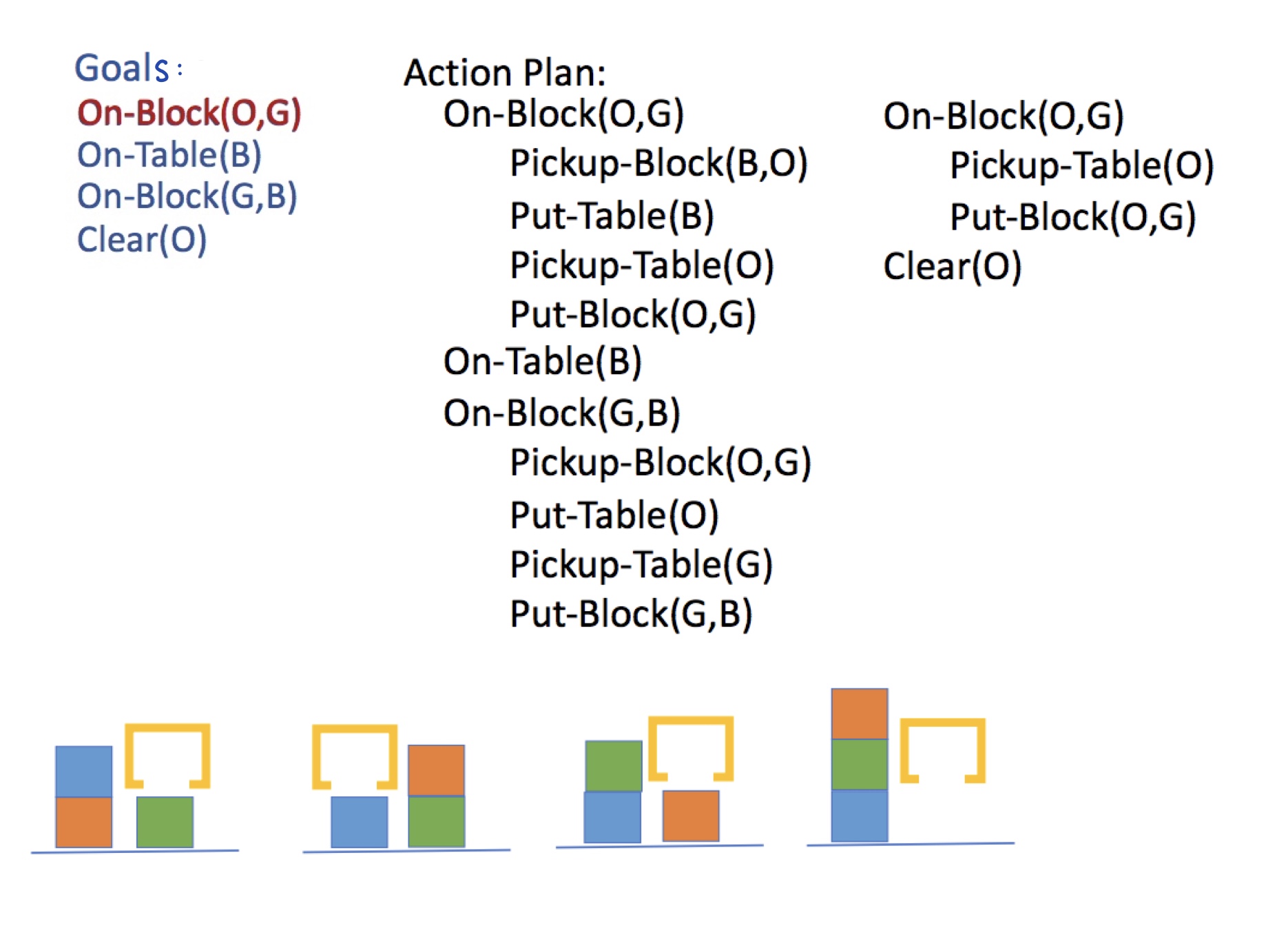
Our goal is On-Block(O, G)\(\wedge\) On-Table(B) \(\wedge\) On-Block(G, B) \(\wedge\) Clear(O). We start by adding all four of these subgoals to a stack and popping them off one by one.

On-Block(O,G): Starting with the first subgoal, we find a plan that involves moving the blue block to the table and then moving the orange block onto the green block.
On-Table(B): Our next subgoal is already achieved because we have already moved the blue block onto the table.
On-Block(G, B): In order to accomplish the third subgoal, we actually have to move the orange block off of the green block in order to move the green block onto the blue block. Thus, we need to push our subgoal On-Block(O,G) back onto the stack.
On-Block(O,G): We can once again move orange back onto the green block.
Clear(O): Orange is clear so this subgoal is already achieved.

Sussman's Anomaly

The above algorithm might not terminate in certain instances. This is due to Sussman's Anomaly, which is when the plan for one subgoal undoes a prior subgoal. We actually saw an example of Sussman's Anomaly earlier when we were trying to find a plan for On-Block(G, B) which violates the subgoal On-Block(O,G). The prior example still terminated. However, in certain cases, we end up switching between the first and second subgoals indefinitely. This issue can occur no matter which subgoal we pick first.

Soundness, Completeness, Optimality

We see that if a plan is found, it is legal, so linear planning is sound. It is not optimal because it might require us to undo some work that we already did. Lastly, linear planning is not complete as illustrated by Sussman's Anomaly.

Contrast with Non-linear planning

Another classical planning algorithm is non-linear planning. Unlike linear planning where we try to achieve one goal at a time, nonlinear planners continually consider a set of subgoals as they put each piece (each operator) together, rather than committing to searching all the way to a selected subgoal.

The pseudocode for a non-linear planning algorithm is shown below:

define NONLINEAR-PLANNING(goals):  
	Initialize set S <- goals  
	While S is not empty:  
		Search different orderings of subgoals to find and select a plan to a subgoal,  
				often with some heuristic for choosing the best option  
		Apply just the first operator of selected plan to subgoal  
		Remove subgoal from S if achieved  
		If a later change violates a subgoal, add it back to S  
	Return plan

Note this pseudocode does not contain the details of the search among subgoals or the heuristic for select the best next step.

For nonlinear planners to be optimal, they would have to consider all possible orderings of subgoals at any given step, which becomes intractable for large planning problems. Instead, they often use heuristics to choose the next step.

Nonlinear planning is also called partial-order planning because it can piece together chains of operations that work in a specific order without necessarily connecting them to the start or the goal state. The algorithms will then figure out which order the chains can be connected to complete the plan.

We see that if a plan is found, it is legal, so nonlinear planning is sound. It is complete, and it could be optimal but we'd have to search all possible inter-leavings. The state-space graphs in the next section expand on why linear and nonlinear planning is so costly.

Planning Representations

State-space graph

A state-space graph (or reachability graph) represents each state as a conjunction of predicates. Edges in the graph represent operators that can be used to move between states. Note that this is not a tree, but a graph; the node at the top is not necessarily the start state.

The start of a state-space graph for Blocks World:

In order to find the goal, we can simply use our regular graph search algorithms such as BFS and DFS. BFS will allow us to find the optimal path to the goal in terms of number of operators. Note that using BFS with a state-space graph is sound (since all solutions found are legal plans), complete (since a solution will always be found if one exists), and optimal (since solutions are found in the order of best to worst).

The downside of using state-space graphs is that the size is exponential in the number of predicates. This is because each predicate can be True or False in one state, and the graph represents all reachable states. Thus, the space complexity is \(2^p\) where \(p\) is the number of predicates. In order to have a more concise representation, we can use the planning graph representation used by the GraphPlan algorithm.

GraphPlan Graph

GraphPlan allows us to reduce the size requirement by using what is called a planning graph. The planning graph alternates between action layers and proposition layers. Proposition layers include all predicates which could be true after executing one action from each action layer. Action layers contain all operators or actions that can be applied given any combination of the true predicates from the layer above it. Edges between predicates and actions represent preconditions. Edges between actions and the next proposition layer represent the effects (making predicates true or false or deleting them).

An interesting note about actions layers is that they also include a "no-op" operator for each predicate in the previous layer. This no-op operator represents doing nothing for each predicate. This is one way to deal with predicates that could persist from one step to the next.

Here is an example of a GraphPlan planning graph for the scenario of eating a cake:

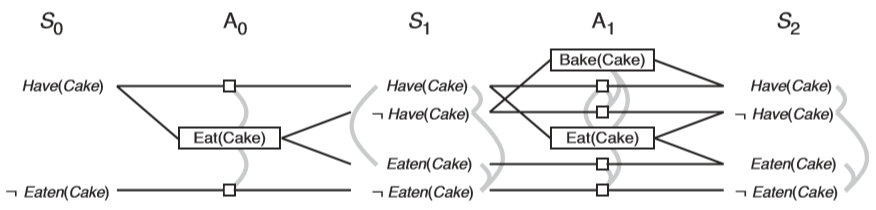
Notice how edges from predicates to operators represent that the propostion is a precondition of the action.

Also notice the grey lines in the example above. These are mutex relations between operators or between propostions to show that they are mutually exclusive. More information about the GraphPlan algorithm can be found in the section below.

The downside of GraphPlan is that it only gives us a heuristic for the number of actions needed to reach the goal. GraphPlan is always correct if it determines that the goal is not reachable. If the goal is reachable, GraphPlan will never overestimate the number of steps. (This is because GraphPlan assumes multiple actions in a single action layer can be taken at once, although in reality these operators must be taken sequentially.) So, the number of actions layers in the final GraphPlan planning graph is an admissible heuristic for the true number of actions needed. The plan extracted from GraphPlan may not be optimal, since there may be a way to reach the goal using more action layers but fewer actions overall.

Note on designing objects, predicates, and operators for GraphPlan graphs: Important: there is a difference between deleting a predicate and adding its negation. We can require as a precondition the negation of a predicate, but we can’t require the absence of a predicate. There are two general strategies for dealing with negations of predicates in GraphPlan (and other planning algorithms).

Explicitly include negations, adding them to the proposition layers. Both the positive and the negated forms of the proposition will often be in the same layer. In this strategy, it is easy to see some of the mutex relationships for negating a precondition or effect of another action and makes it easier to debug. However, it doubles the number of predicates in the proposition layers.
Design predicates to be mutually exclusive by definition in your operators (adding one predicate and deleting another such that only one can be true at a time). This makes it harder to debug and requires more work to determine mutex relationships. However, it is much faster in practice because the branching factor is much smaller.

Remember that we get to design the objects, propositions, and operators, so we can design them to work well with our chosen strategy.

GraphPlan Algorithm

We alternate between graph expansion and mutual exclusion for the GraphPlan Algorithm.

Graph Expansion

We define the very first proposition layer, \(S_0\), as the starting state (all propositions which are true in the beginning).
When adding \(A_t\) after \(S_t\), connect each possible operator in \(A_t\) with their corresponding preconditions in \(S_t\).
When adding \(S_{t+1}\) after \(A_t\), connect each action in \(A_t\) with their effects.

Draw a solid line to predicates that the action adds.
Draw a dotted line to predicates that the action deletes.

Reminder, we also define no-op (no operation) or persist actions from each proposition \(p\) in each action layer \(A_t\), denoted by a square and connecting to the same proposition \(p\) in \(S_{t + 1}\). Below is the same cake example from before.

Actions:

Eat(Cake):

Preconditions: Have(Cake)
Adds: \(\lnot\) Have(Cake), Eaten(Cake)
Deletes: None (we are explicitly including the negation of Have(Cake) rather than deleting it, a design choice)

Bake(Cake):

Preconditions: \(\lnot\) Have(Cake)
Adds: Have(Cake)
Deletes: None

Mutual Exclusion

We start with proposition layer 0. We then expand the graph by adding action layer 0 and proposition layer 1. At this point, we compute mutual exclusion at the action layer and the subsequent proposition layer. One we finish the mutual exclusion, we will expand the graph again (action layer 1 and proposition layer 2), then run mutual exclusion again, etc until the goal predicates are all in the proposition layer and are NOT mutex from each other.

Generally speaking, we define the notion of mutually exclusive (mutex) actions to figure out which actions in the GraphPlan graph would conflict in some way when creating a plan. There are 3 types of mutex relations between two given actions:

Interference: one action's effect deletes or negates a precondition of the other
Inconsistent effects (inconsistency): one action's effect deletes or negates an effect of the other
Competing needs: one action's precondition is the negation of a precondition of the other

Note: It is important to include no-op actions in these mutex relationships.

Proposition will also be mutually exclusive based on the actions that they depend on. Two propositions in proposition layer \(t\) are mutex if:

They are the negation of each other, or
They have inconsistent support. Propositions P and Q in \(S_t\) have inconsistent support if there is no set of non-mutex actions in \(A_{t-1}\) that produce both P and Q.

Exercise: Try to identify what type of mutex relation is specified by each of the gray lines in the cake example above.

Pseudocode

Now that we understand how the graph is constructed, let’s look at the actual GraphPlan algorithm.

# Given a problem and set of goals, returns a plan or NO SOLUTION  
while True:  
	Extend the GraphPlan graph by adding an action level and then a proposition level  
	If no new propositions added from previous proposition level:  
		Return NO SOLUTION (the graph has levelled off)
	If all propositions in the goal are present in the added proposition level:   
		Search for a possible plan in the planning graph  
			(see solution algorithm below)  
		If plan found, return with that plan

Searching for a Possible Plan

First, the search states are the set of propositions in a proposition layer BUT it also includes an additional list of "goals" for that state. The "goals" for this initial state will be the set of planning goals propositions, but as you’ll see below that will change as we search backwards.
Start the search with the initial state being the set of propositions from the last level of the planning graph. We also keep track of the goals for this state, which are the goal propositions for the planning problem. Call this level \(S_t\) for now.
The available search actions are any subset of operators in the preceding action level, \(A_{t-1}\), where none of these actions are conflicting at that level and their collective effects include the full set of goals we are considering in \(S_t\)
Transitions in the search will lead to a next search state with the set of propositions in \(S_{t-1}\) and the "goals" for this state are the preconditions for all of the operators in the search action that was selected.
We keep searching to try to get to \(S_0\), where the "goals" of that search state are all satisfied by \(S_0\).

Using a GraphPlan Solver

In this section we’ll refer to the rocket.py example seen in P3. This section contains all the same information as the "Graphplan Setup" section of the P3 writeup.

Instances are all of the literals and constants in the model. Each Instance has a Type. In the rocket example, London and Paris are Instances of Type PLACE; the rocket is an Instance of Type ROCKET.

Variables can take the value of any Instance of the same Type. For example, in the rocket problem we created a variable

v_from = Variable('from', PLACE)

which can take the value of any possible PLACE instance that we have created. Propositions are boolean descriptors of the environment and act like functions that return a boolean. For example, if the rocket is starting at the instance for London, we might specify that it is ‘at’ London and not ‘at’ Paris.

The states in our problem can be thought of as a set of propositions, or things that are true or false at that given point in time. This means taking an action, i.e. moving from one state to another, is synonymous with adding and/or removing propositions from this list.

To define the start and goal states of the problem at hand, we use lists of Propositions. For instance, the starting state of the Rocket problem is that the package and rocket are at London, and the rocket’s fuel level is 2.

This can be represented as follows:

[Proposition('at', i_package, i_london),     
Proposition('at', i_rocket, i_london),    
Proposition('fuel_at', i_ints[2])]

The goal is for the package to be in Paris, and the rocket to be in London. Note that we do not specify the state of the rocket’s fuel level, so the fuel level can be anything.

Operators contain lists of preconditions, add effects, and delete effects which are all composed of propositions. Operators will test the current state propositions to determine whether all the preconditions are true by matching available instances and/or variables, and if so then add and delete state propositions to update the state.

i_rocket = Instance('rocket', ROCKET)  
i_london = Instance('london', PLACE)  
i_ints = [Instance(0, INT),   
	Instance(1, INT),   
	Instance(2, INT)]

v_fuel_start = Variable('start fuel', INT)  
v_fuel_end = Variable('end fuel', INT)  
v_from = Variable('from', PLACE)  
v_to = Variable('to', PLACE)

o_move = Operator('move',          # The name of the action  
		# Preconditions  
		[Proposition(NOT_EQUAL, v_from, v_to),  
		Proposition('at', i_rocket, v_from),  
		Proposition('fuel_at', v_fuel_start),  
		Proposition(LESS_THAN, i_ints[0], v_fuel_start),  
		Proposition(SUM, i_ints[1], v_fuel_end, v_fuel_start)],  
		
		# Add effects  
		[Proposition('at', i_rocket, v_to),  
		Proposition('fuel_at', v_fuel_end)],  

		# Delete effects  
		[Proposition('at', i_rocket, v_from),  
		Proposition('fuel_at', v_fuel_start)])

In order to perform the move operation, the source must not equal the destination; the rocket must be at the source; the rocket must have v_fuel_start units of fuel such that v_fuel_start > 0 and v_fuel_end + 1 = v_fuel_start.

If the proposition must match the state exactly in the precondition or effects, use an instance. If any instance can be matched, use a variable of the correct type.

For example, one precondition of the "move" Operator is that the rocket’s destination is different from its current location. We can specify this by the Propositions Proposition('at', i_rocket, v_from) and Proposition(NOT_EQUAL, v_from, v_to). Here, we only care about the one rocket Instance’s movement, so we used the i_rocket Instance. As for the PLACE variables, any Variables that satisfy the NOT_EQUAL requirement could be matched (i.e., we could have v_from matched with the London Instance and v_to matched with Paris, or vice versa. Note that whatever v_from is matched to is used throughout the entire Operator. That same Instance must also satisfy the Proposition('at', i_rocket, v_from) precondition, and will be used in the delete effect as well.

After moving, the rocket is now at the destination and has v_fuel_end units of fuel. It is no longer at the source and no longer has v_fuel_start units of fuel. The following image depicts an example of a state that would satisfy the preconditions and be able to move.

This state, however, does not satisfy the preconditions for move, as the starting fuel is not greater than 0.

Important: In GraphPlan, for any proposition named "P", you can't just create another proposition named "notP" and expect that GraphPlan can understand the relationship. GraphPlan would just treat them as two propositions with different names.

It is not a given that "notP" and "P" are mutually exclusive.
Adding "notP" is not equivalent to deleting "P"

Key takeaway: When searching for a plan, GraphPlan considers which actions (operators) to take by trying to match the Variables mentioned with Instances in a way that satisfies the preconditions.