Search: Pre-reading
Search Problem
A search problem is defined by
State Space
For each state s, a set of allowable actions: Actions(s)
Transition Model: Result(s,a)
Step Cost Function: c(s,a,s')
Start State
Goal Test
A solution to a search problem is defined by the sequence of actions from the start to goal state.
Example
State Space

For each state s, a set of allowable actions: Actions(s)
Suppose the agent can rotate 180 degrees clockwise or move forward in the agent's current direction.Actions(A) = {Rotate, Move Forward}
Actions(B) = {Rotate}
Actions(C) = {Rotate}
Actions(D) = {Rotate, Move Forward}Transition Model: Result(s,a)
Result(A, Rotate) = B
Result(A, Move Forward) = C Result(B, Rotate) = A
Result(C, Rotate) = D
Result(D, Rotate) = C
Result(D, Move Forward) = B
Step Cost Function: c(s,a,s')
c(s, Rotate, s') = 1
c(s, Move Forward, s') = 2Start State: A
Goal Test: Is the current state the same as state C?
Search Algorithms
A state space graph is a mathematical representation of a search problem.
Nodes are (abstracted) world configurations
Arcs represent transitions resulting from actions
The goal test is a set of goal nodes
Each state occurs only once
For example, consider the example given for defining a search problem. The corresponding state space graph is below.

We can rarely build this full graph in memory, but it is a useful idea.
Motivation: We can use a search algorithms to find a solution to a search problem. In particular, we can find a path (i.e. sequence of actions) from the start state to the goal state in the state space graph.
Search algorithms can be uninformed search methods or informed search methods.
Tree vs Graph Search
def tree_search(problem):
                initialize frontier as specific work list # (stack, queue, priority queue)
                add initial state of problem to frontier

                while frontier not empty:
                    choose a node and remove it from frontier

                    if node contains goal state:
                        return the corresponding solution

                    for each resulting child from node:
                        add child to frontier

                return failure
def graph_search(problem):
initialize the explored set to be empty
initialize frontier as specific work list # (stack, queue, priority queue)
add intial state of problem to frontier
while frontier not empty:
choose a node and remove it from frontier
if node contains goal state:
return the corresponding solution
add node to explored set
for each resulting child from node:
if child state not in frontier and child state not in explored set:
add child to the frontier
return failure Based on the pseudo-code for tree search vs. graph search, we can see that the main differences are:
Graph search includes an additional explored set to keep track of nodes we have already visited
When adding new nodes to the frontier, graph search will additionally check that the node has not been previously visited (node is not already in the explored set)

Note that the explored set, the frontier, and never seen have no overlaps (no node is added to a frontier if it has been explored, and once a node is popped off of the frontier, it is added to the explored set)
Graph search detects cycles (able to check if a node has already been visited)
Tree search cannot detect cycles (no way of knowing if a node has already been visited)
Uninformed Search Algorithms
Uninformed search methods have no additional information about the cost from the current node to the goal node.

Examples of uninformed search methods include:
Breadth First Search
Depth First Search
Uniform Cost Search
Iterative Deepening
Breadth First Search
Strategy: expand a shallowest node first
Frontier Data Structure: FIFO Queue
Depth First Search
Strategy: expand a deepest node first
Frontier Data Structure: LIFO Stack
Iterative Deepening
Strategy: repeatedly expand a deepest node first (up to a fixed depth)
Frontier Data Structure: LIFO Stack
combines space efficiency of DFS with completeness of BFS
Note: Breadth first search is complete (meaning it will find a path from the start node to the goal node if it exists). In a graph with equal edge weights, breadth first search can be used to find the shortest path from the start node to the goal node. However, depth first search stores less information in the frontier and is therefore more space efficient.
Example
To see these characteristics in action, consider the following graph:
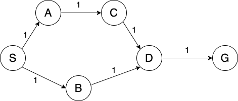
Suppose we run BFS and DFS to find a path from node S to node G (using graph search and breaking ties alphabetically).
BFS
Frontier:
S,S-A,S-B,S-A-C,S-B-D, S-B-D-GExplored Set: S, A, B, C, D
Path: S-B-D-G
DFS
Frontier:
S,S-A, S-B,S-A-C,S-A-C-D, S-A-C-D-GExplored Set: S, A, C, D
Path: S-A-C-D-G
IDS
Limit = 0
Frontier:
SExplored Set: S
Limit = 1
Frontier:
S,S-A,S-BExplored Set: S, A, B
Limit = 2
Frontier:
S,S-A,S-B,S-A-C,S-B-DExplored Set: S, A, C, B, D
Limit = 3
Frontier:
S,S-A,S-B,S-A-C,S-A-C-DExplored Set: S, A, C, D, B
Limit = 4
Frontier:
S,S-A, S-B,S-A-C,S-A-C-D, S-A-C-D-GExplored Set: S, A, C, D
Path: S-A-C-D-G
Notice that BFS returns a shorter path, while DFS has fewer nodes on the frontier. Though DFS found a path to the goal, this is not always the case. We can combine the space-efficiency of DFS with the completeness of BFS. This is the motivation behind iterative deepening.
Uniform Cost Search
Strategy: expand a cheapest node first
Frontier Data Structure: Priority Queue (priority given by cumulative cost)
Note: If we want to find the cheapest path from the start node to the goal node, search algorithms such as BFS and DFS are not guaranteed to give us the right answer. This is where uniform cost search comes in.
Example
Consider the graph from earlier (now with different edge weights):
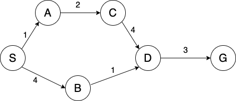
BFS
Frontier:
S,S-A,S-B,S-A-C,S-B-D, S-B-D-GExplored Set: S, A, B, C, D
Path: S-B-D-G
Path cost: 8
DFS
Frontier:
S,S-A, S-BS-A-C,S-A-C-D, S-A-C-D-GExplored Set: S, A, C, D
Path: S-A-C-D-G
Path Cost: 10
IDS
Max Depth = 0
Frontier:
SExplored Set: S
Max Depth = 1
Frontier:
S,S-A,S-BExplored Set: S, A, B
Max Depth = 2
Frontier:
S,S-A,S-B,S-A-C,S-B-DExplored Set: S, A, C, B, D
Max Depth = 3
Frontier:
S,S-A,S-B,S-A-C,S-A-C-DExplored Set: S, A, C, D, B
Max Depth = 4
Frontier:
S,S-A, S-B,S-A-C,S-A-C-D, S-A-C-D-GExplored Set: S, A, C, D
Path: S-A-C-D-G
Path Cost: 10
UCS
Frontier:
(S, 0),(S-A, 1),(S-B, 4),(S-A-C, 3),(S-A-C-D, 7),(S-B-D, 5), (S-B-D-G, 8)Note: Bolded strike through means node was replaced on the frontier. Specifically,
(S-A-C-D, 7)was replaced by(S-B-D, 5). In lecture, we'll introduce this replacement scheme; no need to worry about this just yet.Explored Set: S, A, C, B, D
Path: S-B-D-G
Path Cost: 8
Note: It would be a good idea to go through these search algorithms on your own to see how the frontier, order of the explored set, and path were determined
Search Algorithm Properties
\[\begin{array}{|c|c|c|c|c|}
\hline
\mbox{Algorithm} & \mbox{Time} & \mbox{Space} & \mbox{Complete?} & \mbox{Optimal?} \\ \hline
\mbox{BFS} & O(b^s) & O(b^s) & \mbox{Yes} & \mbox{Yes if edge costs identical} \\ \hline
\mbox{DFS} & O(b^m) & O(bm) & \mbox{Yes if using graph search and search space is finite} & \mbox{No} \\ \hline
\mbox{UCS} & O(b^{\lfloor C^* / \epsilon \rfloor}) & O(b^{\lfloor C^* / \epsilon \rfloor}) & \mbox{Yes (assuming an upcoming modification to graph search)} & \mbox{Yes} \\ \hline
\mbox{Iterative deepening} & O(b^s) & O(bs) & \mbox{Yes} & \mbox{Yes if edge costs identical and using tree search} \\ \hline
\end{array}\]
where
- “depth" / “depth level" of a node = # of edges between the node and the start node
- \(b\) = branching factor, the max number of neighbors each node has.
- \(s\) = the depth level of the shallowest goal node.
- \(m\) = the maximum depth level in the graph.
- \(C^*\) = cost of optimal solution.
- \(\epsilon\) = minimum cost of an edge in the graph.
Brief Explanations
A search algorithm is complete if it finds a path from the start to the goal if one exists.
A search algorithm is optimal if it finds the shortest cost path from the start to the goal.
In some of these explanations we’ll use the term search tree, which is a tree structure illustrating the nodes visited by an algorithm as it searches through the graph.
Note: Other classes you’ve studied these algorithms in may have specified their complexities in terms of the number of vertices/edges in the graph. In AI, we’re more concerned with quantities like \(𝑏\) and \(𝑚\) because it gives a more search agent-centric perspective (e.g., focusing more on the number of actions one can take at a given point).
Note: We’ve provided these explanations just to help establish an intuitive understanding behind the table above. These are in no way a formal proof, but feel free to follow up if you’re interested in something like that.
BFS
Time: BFS will only search up to the depth level of the solution. At worst it'll expand all \(O(b^s)\) such nodes bounded by that depth level:

Space: BFS must keep track of all expanded paths it's considering, which also gets up to \(b^s\) in size.
Completeness: BFS will always terminate because it's guaranteed to find the shallowest goal node, at which point it stops searching.
Optimality: BFS finds the path to the shallowest goal node. If all edges have the same cost, then this path is also the cheapest cost path (and thus the solution found is optimal).
One way to think about BFS is using a priority queue where the priority is the number of edges in the path. You would pull off the path with the smallest number of edges first, so if there are ties, the ties would be broken between paths with the same number of edges. This is NOT an entirely accurate representation of BFS, however, because a priority queue allows you to replace a path already in the queue if you find one with a better priority, which is not representative of the BFS algorithm we use in class, so please use the algorithm presented in class, not a priority queue when running BFS.
DFS
Time: In the worst case, DFS may search all other potential paths in the search tree before finding the solution. The size of this tree is \(O(b^m)\).

Space: Unlike BFS, DFS only keeps the "current" path it's considering on the frontier at a given time. Each level it traverses down the search tree, DFS expands (and adds to the frontier) up to \(b\) nodes, making the space complexity \(O(bm)\).

Completeness: Without keeping track of explored nodes, DFS can get stuck in an infinite loop visiting the same nodes again and again. Thus it only terminates when using graph search.
Optimality: DFS is not optimal. Try to think of a simple example where this is the case.
Similarly to BFS, you could also think of DFS as using a priority queue where the priority is the number of edges in the path, but instead you would pull off the path with the highest number of edges first. Once again, this allows for tie breaking between paths with the same number of edges, but it also has the flaw in that it allows for replacements of paths in the priority queue. Just like BFS, this is NOT an accurate representation of DFS because of this, and it is not representative of the DFS algorithm we use in class, so please use the algorithm presented in class, not a priority queue when running DFS.
UCS
Time: Since UCS follows path costs rather than depth levels, we bound the depth of the optimal solution by \(s \le \lfloor C^* / \epsilon \rfloor\) (as this is the total cost / minimum cost of one edge). Thus it must visit \(O(b^{\lfloor C^* / \epsilon \rfloor})\) nodes.
Space: Similar to BFS, UCS' space complexity is equal to its time complexity because it must keep track of all paths along the current cost contour as it visits nodes.

Completeness: UCS will get stuck in an infinite loop if there is a loop of zero-cost edges, so all edge costs must be \(> 0\).
Optimality: Note that UCS assumes no edges have negative cost - otherwise, it's possible that UCS would exclude an optimal path which has a high positive cost in its earlier edges (but a negative cost later on).
So assuming all edges are non-negative, because nodes are expanded in increasing cost order, when the algorithm gets to a goal node, it must be the lowest cost goal (i.e., must have reached it via the optimal path).
Iterative Deepening
Time: IDS has the same time complexity as BFS, since we are now bounded by the solution's depth level \(s\) (we'll never go deeper than \(s\)).
Space: IDS has the same space complexity as DFS, as we're literally running DFS as a subprocess.
Completeness: Since we're bounded by depth, IDS doesn't fall into the same stuck-in-a-loop trap that DFS does, and will always terminate.
Optimality: IDS also finds the shallowest goal if using tree search (not necessarily graph search - the example used previously serves as a counterexample to this), which is the optimal goal if all edge costs are equal.
Note: While a ton of repeat work is done/space is used in IDS for the lower “failed" depth levels, we can simply consider the work done (space used) at the solution’s depth level (thanks big-O!), because this is where the bulk of the work (space) is, and # of nodes increases exponentially as we go down the search tree.
The time and space complexities of heuristic-based searches depend heavily on the heuristic chosen (surprise, surprise). The listed bounds are worst case scenarios.