School of Computer Science
Carnegie Mellon University
droh@cs.cmu.edu
June 1, 1996
This report summarizes the performance of a family of unstructured finite element simulations of the San Fernando Valley. The simulations were generated by the Archimedes tool chain and run on the Cray T3D at the Pittsburgh Supercomputing Center as part of the Quake project at Carnegie Mellon.
Figure 0 shows the history of the Quake project in terms of largest mesh size as a function of time. After we finished the Archimedes tool chain in the 2nd quarter of 1995, the mesh sizes increased at a rate of about 1 order of magnitude per quarter. The red bars indicate simulations that have been implemented. The blue bar shows the projected size of the ultimate goal, a 1 second simulation of the entire LA Basin.

Figure 0. History of the Quake project (GIF) (postscript)
Section 2 describes Archimedes. Section 3 describes the San Fernando material model. Section 4 describes the unstructured San Fernando finite element models. Section 5 summarizes the performance of four San Fernando simulations on the T3D.
Archimedes is an integrated set of programs for building unstructured finite element models and simulating them on parallel computers. The basic idea is shown in Figure 1. The programs on the left hand side (Triangle, Pyramid, Slice, and Parcel) generate the unstructured finite element model from an initial description of the geometry of the domain. The programs on the right hand side (Author, the Archimedes runtime library, and the native C compiler) generate the parallel code that simulates the model from a sequential C-like description of the finite element algorithm. The Archimedes tools run on any Unix system with a C compiler. The parallel finite element simulations generated by Archimedes run on any parallel or distributed system with a C compiler and an MPI implementation.

Figure 1. The Archimedes tool chain (GIF) (postscript)

Figure 2. Plane view (GIF) (postscript)

Figure 3. Cross section A1-A2 (GIF) (postscript)

Figure 4. Cross section B1-B2 (GIF) (postscript)
Figure 4 summarizes the family of San Fernando finite element models. Each models comprises an identical volume of 50km x 50km x 10km, and resolves waves up to some frequency. Roughly speaking, mesh sfk is sufficiently fine to resolve a wave with a period of k/2 seconds, under the assumption of 10 mesh nodes per wave.
| Nodes | Equations | Elements | Edges | |
|---|---|---|---|---|
| sf10 | 7,294 | 21,882 | 35,025 | 44,922 |
| sf5 | 30,169 | 90,507 | 151,173 | 190,377 |
| sf2 | 378,747 | 1,136,241 | 2,067,739 | 2,509,064 |
| sf1 | 2,461,694 | 7,385,082 | 13,980,162 | 16,684,112 |
Figure 5. Summary of San Fernando models.
Figures 6-9 show the process of generating an Archimedes simulation, using the sf5 model as a running example. First, an octree-based algorithm samples the material model to scatter nodes in the domain, as shown in Figure 6. Notice that regions of soft soil with slower shear wave velocities need a higher concentration of nodes to resolve the shorter wavelengths associated with soft soils.

Figure 6. sf5 nodes (GIF) (postscript)
Pyramid uses the node set in Figure 6 to produce the 3D mesh in Figures 7 and 8. Notice that the volumes of the different elements can differ by several orders of magnitude, reflecting the wide variance in the density of the soil and the corresponding wavelengths

Figure 7. sf5 mesh (side view) (GIF) (postscript)

Figure 8. sf5 mesh (top view) (GIF) (postscript)
Slice partitions the 3D mesh into subdomains, as shown in Figure 9. The particular partition in Figure 9 consists of 64 subdomains, each denoted by a different color.

Figure 9. sf5 partition (64 subdomains) (GIF) (postscript)
Parcel then reades the partitioned mesh to produce a single pack file, which contains the global to local mapping of nodes and elements for each subdomain, attributes for each node and element, the sparsity structure of the matrices in each subdomain, and the communication schedule for each subdomain. The communication schedule for the 64-subdomain partition is shown in Figure 10. Each vertex in the graph corresponds to a subdomain, and each edge corresponds to communication between subdomains.

Figure 10. sf5 communication graph (64 PE's) (GIF) (postscript)
Figure 11 shows the running times for the San Fernando family of meshes (excluding the initial file input) as a function of the number of T3D processing elements (PE's). The largest simulation, sf1, requires about 1.5 hours to simulate 60 seconds of shaking on 128 PE's.

Figure 11. Running time on Cray T3D. (GIF) (postscript)
Figure 12 gives the computation/communication breakdown for the sf2 simulation during its main loop as a function of the number of PE's. Between 80-90% of the time is spent performing local computation (primarily local calculation of boundary conditions, local matrix-vector products, and local vector-vector sums and products). Only 10-20% of the time is spent exchanging data among PE's, and this communication occurs only during the global sparse matrix vector product operations. The relatively small amount of communication time is the first hint that the simulations scale well.

Figure 12. Performance breakdown for the sf2 main loop. (GIF) (postscript)
Figure 13 breaks down the performance from a different angle: how much time is spent performing vector-vector sums and products (5%), computing boundary conditions (15%), and performing global sparse matrix vector product operations (80%). Clearly, the sparse matrix vector product operations dominate the running time.

Figure 13. Functional performance breakdown for the sf2 main loop. (GIF) (postscript)
Figure 14 shows the MFLOPS per PE sustained during the sparse matrix-vector product operations as a function of the number of PE's. The smaller simulations run out of work on larger numbers of PE's. However, the larger simulations are able to sustain rates of roughly 25 MFLOPS per PE. These rates are attained with compiler generated C code. No assembly language tuning was necessary.

Figure 14. MFLOPS per PE during main loop on the Cray T3D. (GIF) (postscript)
Figure 15 shows the aggragate MFLOPS rate sustained by the entire family of simulations during the sparse matrix vector product operations as a function of the number of PE's. The largest simulation sustains an aggragate rate of over 3 GFLOPS.

Figure 15. Aggregate MFLOPS on the Cray T3D. (GIF) (postscript)
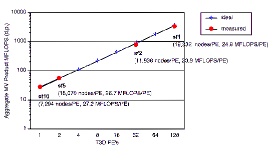
Figure 16 shows how the sustained aggragate MFLOPS rate of the inner loop scales with the number of PE's when the number of nodes per PE (and thus the amount of work on each PE) is roughly constant. As the graph shows, the MFLOPS rate scales linearly with the number of PE's.

Figure 16. Scaling with respect to MV-product MFLOPS. (GIF) (postscript)
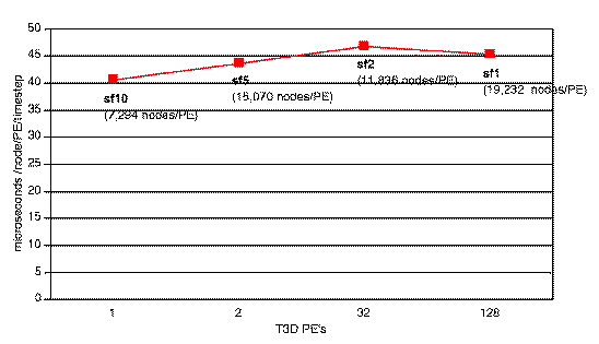
The truest measure of scalability is the actual running time. Figure 17 shows the time per node per PE per timestep when the number of nodes per PE is roughly constant. As the graph shows, this time is constant to within 10%, and the difference is accounted for by the fact that we are not able to get the number of nodes per PE exactly equal for the different simulations.

Figure 17. Scaling with respect to running time. (GIF) (postscript)
The results in Figure 17 suggest that both the underlying solution methodology and the code generated by Archimedes scale well with increasing problem size. This is a significant and encouraging result, suggesting that a high frequency simulation of the entire LA Basin, roughly 10x the size of the 1-second San Fernando simulation, is within reach.