
fft2(), and then zero'd out a black square in the middle of this frequency representation. The resulting frequency-domain image looked like this:
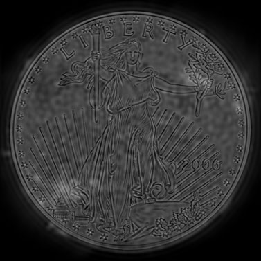
I then transformed this frequency-domain image back into the spatial domain. The resulting image looked like this:

This image shows only the high frequencies of the original photo, which was the expected output since the black square in the middle of the frequency representation removed the low-frequency content.
Instead of drawing a square to attenuate a range of frequencies, the output could be improved by using a gaussian distribution. Thus the next step was to create a function to generate a gaussian circle. To this end, I wrote gaussCircle() (wrapping MATLAB's gaussmf()) which accepts an argument to define the cutoff frequency, and another argument to specify a 'soften' factor to control the softness of the circle edges (thus controlling how quickly the frequencies are attenuated). An example of gaussCircle() is:

The process to generate a hybrid image was fairly simple once the gaussian-circle code was in place. The total process can be summarized in 7 steps:
(1) convert the input images to grayscale
(2) align the input images (resulting in equal dimensions)
(3) create two gaussian circles: one for the low-frequency content, and the other for the high-frequency content (e.g.,  and , respectively)
(4) convert the input images to the frequency domain (via fft2())
(5) multiply the frequency-domain images by their respective gaussian circles (which removes low-frequency content in one, and high-frequency content in the other)
(6) convert the frequency-domain images back into the spatial domain (via ifft2())
(7) combine the spatial-domain images by doing an element-wise average

The images below illustrate the process of creating this hybrid image.

Above are the two input images.

Above is is the log magnitude of the two frequency-domain input images. (The left side is the first input image, and the right side is the second input image.)

Above is the log magnitude of the two frequency-domain images after applying their respective gaussian-circle masks. (The left side is the low-frequency component, and the right side is the high-frequency component.)

Above are the spatial-domain images after applying their respective gaussian-circle masks in the frequency domain, to remove the high-frequency content (left side) and the low-frequency content (right side).

Above is the log magnitude of the frequency-domain hybrid image.
 +
+
 =
=

 +
+
 =
=
 +
+
 =
=
