Bayesian Color Constancy for Outdoor Object Recognition

Yanghai Tsin, Robert Collins, Visvanathan Ramesh and Takeo Kanade

Appears In IEEE Computer Vision and Pattern Recognition (CVPR)
2001, Kauai, Hawaii
The paper is available at the RI publication page

Abstract
Outdoor scene classification is challenging due to irregular geometry, uncontrolled illumination, and noisy reflectance distributions. This paper discusses a Bayesian approach to classifying a color image of an outdoor scene. A likelihood model factors in the physics of the image formation process, the sensor noise distribution, and prior distributions over geometry, material types, and illuminant spectrum parameters. These prior distributions are learned through a training process that uses color observations of planar scene patches over time. An iterative linear algorithm estimates the maximum likelihood reflectance, spectrum, 
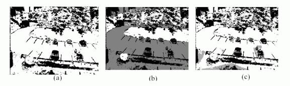
geometry, and object class labels for a new image. Experiments on images taken by outdoor surveillance cameras classify known material types and shadow regions correctly, and flag as outliers material types that were not seen previously.


Figure 1. (a) A sample input image and the small scene patch selected for training the algorithm. (b) The mean color chart. The first row represents colors of the road pavement under different lighting source, and the second row represents mean colors of the vegetation. The three lighting sources (from left to right) are: early morning, shadow, and sunlight (c) Original image patches under the three lighting sources. Notice the similarity between the image patch and the corresponding mean color, and the obvious color difference under different lighting sources.


Figure 2. (a) The relative median error as a function of the number of basis functions. (b) Scatter plot for the two surface types of 
interest. (c) Illuminant spectrum clusters


Figure 3. Initial segmentation based on comparison with the mean color chart. (a) The test image. (b) Initial segmentation by material types. White: vegetation. Gray: road pavement. (c) Initial segmentation by lighting source. White: sunlight. Gray: shadow. Dark gray: early morning

Figure 4. Final results. (a) The detected outliers. Outliers are shown as black pixels (b) Final segmentation by material types. White: vegetation. Gray: road pavement. (c) Final segmentation by lighting source. White: sunlight. Gray: shadow.