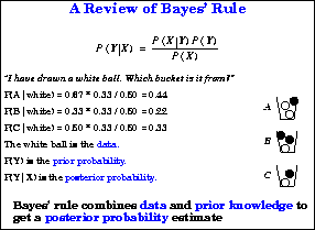
Figure 21: An illustration of Bayes' rule
Regression analysis can have a serious problem if there is not enough data present. The immediate result of insufficient data is that the matrix being inverted in eq. 8 becomes singular and the inversion fails. That means the data is insufficient to determine all the coefficients in the regression.
This problem shows up frequently when using locally weighted regression for decision making. The local weighting is part of the problem. It is possible to have a fairly large data set, but still make queries that fall well outside the regions covered by the data. In that case, the weighting function will weight all the data near zero and the situation will be just like the case where there really is no data. One scenario where this happens is when a controller is considering the potential affects of choosing a control decision that has never been tried before. Since it's never been tried before there is little or no data to estimate what will happen. Another scenario is when a decision is being made about what data to collect. Often, the best place to collect data is where there is not much data already and making queries on the model to find these places will cause the insufficient data problem to show up.

Figure 21: An illustration of Bayes' rule
Bayesian regression can be used to avoid the insufficient data problem. It allows us to easily specify prior information about what values the coefficients should have when there is not enough data to determine them. To see how Bayesian regression works, we first review Bayes' rule with a simple example (see fig. 21). The important thing to understand about Bayes' rule is that it combines prior information (initially there is an equal chance of choosing from any bucket), with data (the chosen ball was white) to obtain a posterior estimate (that the probability of buckets A, B, and C is 0.44, 0.22, 0.33).
With Bayesian regression we specify a joint prior distribution on the coefficients and the noise called a normal-gamma distribution. The prior distribution on the inverse of the variance of the noise is a gamma distribution and the prior on the coefficients given a particular level of noise is a normal (Gaussian) distribution. Bayesian regression provides us with a way to combine those priors with the data to yield the posterior distributions on the coefficients and the noise described in the last section. The details are described in a text by DeGroot [3].

Figure 22: Example with Bayesian locally weighted regression. See text for
explanation

Figure 23: Example with Bayesian locally weighted regression. See text for
explanation
Fig. 22 shows one example of what using Bayesian locally weighted regression does. The plot at the lower left shows a data set we are modeling. The plot above it shows the first few data points. The large plot on the right shows the distributions of the predicted outputs as more data points are included. The curves are like the 0-d prediction distributions we saw earlier. The lowest curve is the prior distribution for the output at a query of 0.47, which is what we get if we ask for a prediction at that point without giving it any data points. You can see what this looks like in Vizier by loading the data file empty.mbl. You'll have to rescale the axes to get a plot like the one in the figure. The next higher curve is obtained by giving it only one of the data points from the upper left hand plot. The next curve is from two data points. The distribution is gaining a slight hump around 0.8. Even with two data points, there is still not enough information to complete the regression using the basic regression method of eq. 8. It is the fact that we are using Bayesian methods, that allows the curves to be drawn. Finally, when the third data point is included, there is enough evidence to show some confidence in the output at input 0.47. Even with these three data points, though, the distribution shows that we shouldn't be surprised if the true mean output at input 0.47 is as low as 0.0 or as high as 2.0. Finally, the last curve shows what the distribution looks like after all 100 data points are included. The model is very confident that the true output at input 0.47 lies between 0.7 and 1.2.
Fig. 23 is another example demonstrating Bayesian regression
in action. In this example, there are two input variables (labeled x
and y) and one output variable (labeled z). There are only two
data points as pointed out in the plot at the top. We want to fit a linear
model to the data, but these two points are insufficient. Using Bayesian
regression allows us to finish the computation and get reasonable confidence
intervals anyway. Suppose we are interested in the gradient at the query
half way between the two data points (we would like to know ![]() and
and ![]() at the point (0.3,0.6)). The plot at the lower left
shows what these two distributions look like. Since the two data points
are aligned horizontally, we can make a good estimate of
at the point (0.3,0.6)). The plot at the lower left
shows what these two distributions look like. Since the two data points
are aligned horizontally, we can make a good estimate of ![]() and the distribution shows that it is probably between 2.0 and 3.0. There
is no information in the y direction, though, and the distribution for
and the distribution shows that it is probably between 2.0 and 3.0. There
is no information in the y direction, though, and the distribution for
![]() show great uncertainty with only a slight preference for a
derivative near zero. Now suppose we want to make a prediction of the output
at the query (0.8,0.6). Since the query is aligned with the data points,
we get a relatively confident prediction. However, if we query at (0.3,0.3),
the prediction is unconfident with only a slight preference in the range of
outputs from the two existing data points.
show great uncertainty with only a slight preference for a
derivative near zero. Now suppose we want to make a prediction of the output
at the query (0.8,0.6). Since the query is aligned with the data points,
we get a relatively confident prediction. However, if we query at (0.3,0.3),
the prediction is unconfident with only a slight preference in the range of
outputs from the two existing data points.
These two examples show some of the benefits of using Bayesian locally weighted regression. The main thing to remember about it is that we don't have to worry about the problem of insufficient data. The computation completes without any numeric difficulties, and we get wide confidence intervals when we ask questions for which there isn't enough data to support a good answer.