To set up the equations lets consider a particular cell. The flow
into the cell is the sum of the flow through its edges. We already
mentioned that each of the cell's edges is associated with another
point. Based on equation 3 we would like to determine the
gradient of ![]() along each edge in a direction perpendicular to the
edge. This gradient can be determined to a good approximation by
taking the difference in the value of
along each edge in a direction perpendicular to the
edge. This gradient can be determined to a good approximation by
taking the difference in the value of ![]() at the two points
associated with the edge and dividing this difference by the distance
between the points (a gradient is simply a directional first
derivative, i.e. a slope). Note that the line joining the two points
is perpendicular to the edge. To approximate the flow across
the edge we then simply take this gradient and multiply it by
the length of the edge. For example, consider the following cells:
at the two points
associated with the edge and dividing this difference by the distance
between the points (a gradient is simply a directional first
derivative, i.e. a slope). Note that the line joining the two points
is perpendicular to the edge. To approximate the flow across
the edge we then simply take this gradient and multiply it by
the length of the edge. For example, consider the following cells:
The flow through the edge e-n into cell ![]() is
is ![]() , where
, where ![]() is the length of an edge.
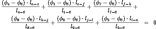
Now to generate our linear equation for the cell we simply add up all
the flows into the cell and set this sum to zero. For the above example
the equation for cell
is the length of an edge.
Now to generate our linear equation for the cell we simply add up all
the flows into the cell and set this sum to zero. For the above example
the equation for cell ![]() would be
would be
We could write similar equations for each of the nine points (cells) in the diagram. This would give us a set of equations of the form
![]()
where the ![]() would be a sparse matrix with the coefficients of
our equations, the vector
would be a sparse matrix with the coefficients of
our equations, the vector ![]() would be the values of
would be the values of ![]() at each point,
which we are trying to solve for, and the vector
at each point,
which we are trying to solve for, and the vector ![]() would be all 0s.
would be all 0s.
The one thing we have not considered are the boundary conditions.
Earlier we discussed how we assume that the flow through the surface
of any object is 0. To deal with this we don't have to
do anything special. For example, for cell 3 in the above diagram, if
we say that the sum of the flows through edges ![]() ,
, ![]() and
and ![]() is 0 then we are implicitly assuming that the flow through the
boundaries
is 0 then we are implicitly assuming that the flow through the
boundaries ![]() and
and ![]() is 0. Also as mentioned earlier we assume
that the flow through the top and bottom of our space is 0. This
can be dealt with in a similar way.
is 0. Also as mentioned earlier we assume
that the flow through the top and bottom of our space is 0. This
can be dealt with in a similar way.
The only two tricky boundary conditions we have to consider are the
left and right hand sides of our space. To deal with the left side
we set the flow through the boundary to a value that is proportional
to the component of the boundary parallel to the ![]() axis. For example,
the equation for cell 2 would be:
axis. For example,
the equation for cell 2 would be:
![]()
where ![]() is the sum of the
flow through edges
is the sum of the
flow through edges ![]() and
and ![]() . In the assignment
we are going to give you these sums for each point on the left boundary.
. In the assignment
we are going to give you these sums for each point on the left boundary.
To deal with the right boundary we set ![]() to zero
on each of these points. We can do this by using
the equation
to zero
on each of these points. We can do this by using
the equation ![]() for each
for each ![]() along the right boundary instead
of using our equation based on flow into the cell.
along the right boundary instead
of using our equation based on flow into the cell.