FFT Based Procedure for Texture Synthesis

Xuewen Chen

xuewen@andrew.cmu.edu

1. INTRODUCTION

Texture synthesis has been a widely studied area in compute vision and computer graphics. It has been applied to broad fields such as image modeling, graphics and hole filling. The primary approach for texture synthesis has been to develop a statistical model which emulates the generative process of the texture they are trying to mimic. For example, Zhu et al [1] use a Markov random field (MRF) to model texture with some success. Heeger and Bergen [2] resample a random noise image to coerce it into a texture sample with similar histograms. It works well for highly stochastic textures, but fails for more structures textures.

Most recently, Efros and Leung [3] propose a very simple algorithm based on MRF without estimate of specific distribution. Their paper presents many impressive 2D textures and demonstrates that simple method do work well. However, as they mentioned in their paper, the algorithm is quite slow.

In this paper, we propose an efficient algorithm based on their algorithm. We will use fast Fourier transform technique (FFT) to search matching points. We provide a theoretical analysis by comparing the computation needed in both algorithms. Our results show that using FFT based algorithm will perform much faster than their algorithm, especially when the matching window has a large size, which is needed for most texture synthesis.

2. Previous work

In Efros and Leung’s work, textures are assumed to satisfy MRF, i.e, the probability distribution of intensities for each pixel given the intensities of its spatial neighborhood is independent of the rest of the texture image. Therefore, to synthesize a pixel for new texture image, a window centered in this pixel is formed and a sum of squared differences (SSD) is used to find all neighborhoods in sample image that are similar to the pixel’s neighborhood. A histogram is then formed from all matching pixels in sample image. The new synthesized pixel is simply sampled from the histogram. In this algorithm, an important parameter specified by user is the matching window size. A small window may not capture the necessary features of textures.

Given a sample texture image, a new image is synthesized one pixel at a time. This is one of two main reasons that make this algorithm to be slow. The other reason is that: to synthesize one pixel, we have to calculate all possible SSDs between pixels around the new pixel (within a matching window) and corresponding pixels around each pixel (local window with same window size as matching window) in sample image. Assuming that the sample image A has size of M ´ N and the matching window B has size of m ´ n. To synthesis a texture image, we will need about M ´ N ´ (M ´ N ´ 4 ´ m ´ n + m ´ n) computations. For example, for a 100 x 100 sample image and 20 ´ 20 matching window, we need about 1.6´10¹¹ computations. This is a very large number.

To speed up, we have to reduce the computation time. In section 3, we will describe a new strategy to compute SSD efficiently so as to reduce the number of operations.

3. FFT based algorithm

The way to compute SSDs can be viewed as convolutions. Thus, instead of computing SSD pixel by pixel in sample image, we first zero pad image A and matching window B to the same size of (M + m –1) ´ (N + n –1). Then we perform FFT of the zero paded A and B and the inverse FFT of multiplication of their Fourier transform [4]. To synthesis a texture image, we will need total M ´ N ´ (2 ´ 3 ´ (M + m –1) ´ (N + n –1) ´ (log₂(M + m –1) + log₂(N + n –1) ) + m ´ n) computations, which, as we will show, is much smaller than the number needed in Efros and Leung’s algorithm for larger window size.

To see the computation reduction, we plot the number of computations vs. window size m (here for simplicity, we assume m = n, M = N = 100). As seen from figure 1, as the window size increases, the number of computations needed for Efros’ algorithm increases dramatically compared with my algorithm. To see this clear, I also plot the log₁₀(number of computation) vs. m. It is clear that for m between 10 and 30, my algorithm is about 10 times faster than Efros’, and for m large than 50, my algorithm will run about 100 times faster than Efros’ algorithm. Therefore, we cam reduce the computation time dramatically. Only for m equal to 3 and 4, Efros’ algorithm performs faster than my algorithm. However, as I will demonstrate, it is impractical to use so small window, which may not find the undergoing stochastic property (This is also discussed in Efros’s paper).

Figure 2

To have an idea about how large the matching window should be, we test our algorithm for synthesizing brick texture. Figure 3(a) is the sample texture, and 3(b) – (d) are synthesized textures with matching window size of 5 ´ 5, 15 ´ 15, and 31 ´ 51, respectively. Obviously, in this case, as window size is larger and larger, the results are better and better.

(a) (b) (c) (d)

figure 3 (a) sample texture, (b), (c), and (d) synthesized textures with 5 x 5, 15 x 15, and 31 x 51 window sizes, respectively.

4. SELECTED Results and Discussion

In this section, I will present more synthesis results using my algorithm. In figures 4-8, (a) is the sample texture, (b) is the results from Efros and Leung, and (c) is the results from my algorithm. Note that the synthesized textures from Efros’ algorithm and my algorithm have different sizes (I do not know the size of their synthesized texture), and some parameters used are different either (If I have more time, I may find better parameters for each case and obtain better results).

Figure 4-6 show the synthesized textures from sample images using Efros’ and my algorithm. As we can see, the results are very similar , although we use different parameters such as window sizes and Gaussian weights (I found that Gaussian weights used in SSDs are also an important parameters).

(a) (b) (c)

figure 4

(a) (b) (c)

figure 5

(a) (b) (c)

figure 6

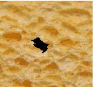
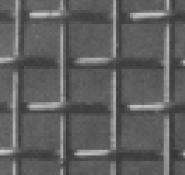
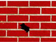
Figure 7-9 show the results from hole filling by using my texture synthesis algorithm. As can be seen, the filled holds represent the texture sample very well (It only takes less than 1 minute to fill these holes).

(a) (b)

figure 7 (a) texture with hole (b) filled hole

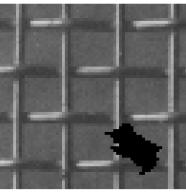
(a) (b)

figure 8 (a) texture with hole (b) filled hole

(a) (b)

figure 9 (a) texture with hole (b) filled hole

5. FUTURE WORK AND IMPROVEMENTS

In this paper, we only reduce the computation time for searching matching pixels. To further reduce the computation time, we can try to synthesis a patch instead of one pixel each time.

Another issue is the window size. It is very important to select a proper window size. An automatic selection of window size will be desired. We may consider a moving average (MA) model together with MRF to model the intensity of each pixel. The size of MA window is the same as the matching window. When we increase the window size, the error (difference between real intensity and intensity estimated from MA model) will decrease. When the difference is small enough, the corresponding window size may be used as matching window size.

6. REFERENCE

[1] S. C. Zhu, Y. Wu, and D. Mumford, "Filters, random fields and maximum entropy" International Journal of Computer Vision, vol. 27(2), pp.1-20, 1998.

[2] D. J. Heeger and J. R. Bergen, “Pyramid based texture analysis/synthesis” in Computer Graphics, pp. 229-238, ACM SIGGRAPH, 1995.

[3] A. A. Efros and T. K. Leung, “Texture synthesis by non-parametric sampling” IEEE International Conference on Computer Vision (ICCV’99), 1999

[4] A. K. Jain, Fundamentals of digital image processing, Prentice-Hall, Inc., 1989.