Stationary probabilities

We first discuss some key properties of the stationary probabilities in a QBD process. Consider a simpler case of the birth-and-death process having the generator matrix shown in (3.1). Let $\pi_\ell$ be the stationary probability that the birth-and-death process is in level $\ell$ for $\ell\geq 0$. Then, it is easy to see that $\pi_{\ell} = \rho_\ell\pi_{\ell-1}$, where $\rho_\ell = \frac{f_{\ell-1}}{b_{\ell}}$, for $\ell\geq 0$. It turns out that the stationary probabilities in a QBD process have a similar property. Let $\Vec{\pi_\ell}$ be the stationary probability vector in a QBD process having generator matrix shown in (3.2). Here, the $i$-th element of vector $\Vec{\pi_\ell}$ denotes the stationary probability that the QBD process is in phase $i$ of level $\ell$, i.e. state ($i,l$). It turns out that there exists a matrix $\mathbf{R}^{(\ell)}$ such that $\Vec{\pi_{\ell}} = \Vec{\pi_{\ell-1}} \mathbf{R}^{(\ell)}$ for each $\ell\geq 1$.

Specifically, the stationary probability vector in the QBD process is given recursively by

$$\Vec{\pi_\ell} = \Vec{\pi_{\ell-1}} \mathbf{R}^{(\ell)},$$ (3.3)

where $\mathbf{R}^{(\ell)}$ is given recursively via:

$$\mathbf{F}^{(\ell-1)} + \mathbf{R}^{(\ell)} \mathbf{L}^{(\el... ...ll)} \mathbf{R}^{(\ell+1)} \mathbf{B}^{(\ell+1)} = \mathbf{0}.$$ (3.4)

When the QBD process has an infinite number of levels, the state space of the QBD process needs to be truncated, so that $\mathbf{R}^{(\ell)}$ matrices can be calculated from a certain large enough integer $\ell=L$ to $\ell=1$ recursively via (3.4). The truncation level $L$ needs to be chosen carefully such that the stationary probability that the QBD process is above level $L$ is negligible [28].

When the QBD process repeats after a certain level, $\hat\ell$, (i.e., $\mathbf{F}^{(\ell)} = \mathbf{F}$, $\mathbf{L}^{(\ell)} = \mathbf{L}$, and $\mathbf{B}^{(\ell)} = \mathbf{B}$ for all $\ell\geq\hat\ell$), $\mathbf{R}^{(\ell)}$ is the same for all $\ell>\hat\ell$, and $\mathbf{R}=\mathbf{R}^{(\ell)}$ (for $\ell>\hat\ell$) is given by the minimal nonnegative solution to the following matrix quadratic equation^3.3:

$$\mathbf{F} + \mathbf{R} \mathbf{L} + (\mathbf{R})^2 \mathbf{B} = \mathbf{0}.$$ (3.5)

Once $\mathbf{R}^{(\hat\ell+1)} = \mathbf{R}$ is obtained, $\mathbf{R}^{(\ell)}$ for $1\leq \ell \leq \hat{\ell}$, is given recursively via (3.4). Various approaches for calculating $\mathbf{R}$ have been proposed, and in Figure 3.12 we show an algorithm for calculating $\mathbf{R}$, $\mathbf{R}^{(\ell)}$'s, and other relevant matrices.

Figure: Algorithms for calculating $\mathbf{R}$, $\mathbf{R}^{(\ell)}$'s, and other relevant matrices [111]. The input matrices ($\mathbf{R}$, $\mathbf{G}$, and $\mathbf{U}$) for part (b) are given by the output of part (a).

Input: $\mathbf{F}$, $\mathbf{L}$, $\mathbf{B}$, $\epsilon$

Output: $\mathbf{R}$, $\mathbf{G}$, $\mathbf{U}$

$\mathbf{H} = (-\mathbf{L})^{-1} \mathbf{F}$;

$\mathbf{K} = (-\mathbf{L})^{-1} \mathbf{B}$;

$\mathbf{G} = \mathbf{K}$;

$\mathbf{T} = \mathbf{H}$;

repeat

$\mathbf{U} = \mathbf{H}\mathbf{K} + \mathbf{K}\mathbf{H}$;

$\mathbf{M} = (\mathbf{H})^2$;

$\mathbf{H} = (\mathbf{I}-\mathbf{U})^{-1} \mathbf{M}$;

$\mathbf{M} = (\mathbf{K})^2$;

$\mathbf{K} = (\mathbf{I}-\mathbf{U})^{-1} \mathbf{M}$;

$\mathbf{G} = \mathbf{G} + \mathbf{T}\mathbf{K}$;

$\mathbf{T} = \mathbf{T}\mathbf{H}$;

until $\vert\vert\Vec{1} - \mathbf{G}\Vec{1}\vert\vert _{\infty} \leq \epsilon$

$\mathbf{U} = \mathbf{L} + \mathbf{F}\mathbf{G}$;

$\mathbf{R} = \mathbf{F} (-\mathbf{U})^{-1}$;

Input: $\mathbf{R}$, $\mathbf{G}$, $\mathbf{U}$

Output: $\mathbf{R}^{(\ell)}$'s, $\mathbf{G}^{(\ell)}$'s, $\mathbf{U}^{(\ell)}$'s

$\mathbf{U}^{(\hat\ell+1)} = \mathbf{U}$

$\mathbf{G}^{(\hat\ell+1)} = \mathbf{G}$

$\mathbf{R}^{(\hat\ell+1)} = \mathbf{R}$

for $\ell=\hat\ell$ to 1

$\mathbf{U}^{(\ell)} = \mathbf{L}^{(\ell)} + \mathbf{F}^{(\ell)} \mathbf{G}^{(\ell+1)}$

$\mathbf{G}^{(\ell)} = (-\mathbf{U}^{(\ell)})^{-1} \mathbf{B}^{(\ell)}$

$\mathbf{R}^{(\ell)} = \mathbf{F}^{(\ell-1)} (-\mathbf{U}^{(\ell)})^{-1}$

end

(a) repeating part

(b) nonrepeating part

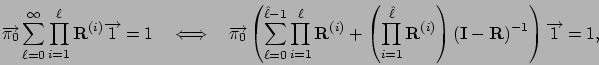
Once $\mathbf{R}$ and $\mathbf{R}^{(\ell)}$'s are obtained, the stationary probability vector $\Vec{\pi_\ell}$ can be calculated recursively from $\Vec{\pi_0}$ via (3.3) for $\ell\geq 1$. Thus, all that remains is to calculate $\Vec{\pi_0}$. Vector $\Vec{\pi_0}$ is given by a positive solution of

$$\Vec{\pi_0} \left(\mathbf{L}^{(0)} + \mathbf{R}^{(1)} \mathbf{B}^{(1)}\right) = \Vec{0},$$

normalized by the equation

$$\Vec{\pi_0}\sum_{\ell=0}^\infty \prod_{i=1}^\ell \mathbf{R}^... ...(i)}\right) (\mathbf{I}-\mathbf{R})^{-1} \right) \Vec{1} = 1,$$

where $\Vec{0}$ and $\Vec{1}$ are vectors with an appropriate number of elements of 0 and 1, respectively.