The following steps allow us to obtain the moments of
![]() :
:
 ,
because the queue reaches the stationary state.
Now,
,
because the queue reaches the stationary state.
Now,
(i) We first set up a differential equation for
![]() . For this purpose, we carefully
examine the relationship between
. For this purpose, we carefully
examine the relationship between ![]() and
and ![]() .
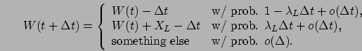
First, suppose
.
First, suppose
![]() (see Figure A.1(a)).
Since the long server is always busy between
(see Figure A.1(a)).
Since the long server is always busy between ![]() and
and ![]() ,
only long jobs could arrive at the queue.
Since the arrival process is Poisson with rate
,
only long jobs could arrive at the queue.
Since the arrival process is Poisson with rate ![]() ,
the probability of having a job arrival in time
,
the probability of having a job arrival in time ![]() is
is
![]() .
Any such arrival will have service time
.
Any such arrival will have service time ![]() .
Therefore,
.
Therefore,
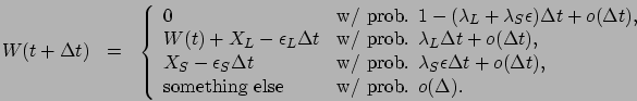
Next, suppose
![]() (see Figure A.1). Let a random variable
(see Figure A.1). Let a random variable ![]() be the fraction of time that the long server was idle during
be the fraction of time that the long server was idle during
![]() given that there were no arrivals during this interval.
Let a random variable
given that there were no arrivals during this interval.
Let a random variable ![]() be the fraction of time that the
long server was busy during this interval given that there was a long job
arrival. Let a random
variable
be the fraction of time that the
long server was busy during this interval given that there was a long job
arrival. Let a random
variable ![]() be the fraction of time that the long server
was busy during the interval giving that there was a short job arrival.
Then,
be the fraction of time that the long server
was busy during the interval giving that there was a short job arrival.
Then,
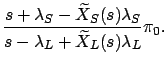
Based on the above observation, the Laplace transform
![]() of
of ![]() is obtained as follows:
is obtained as follows:
![$\displaystyle \int_{x=0}^\infty \mbox{{\bf\sf E}}\left[ e^{-sW(t+\Delta t)}\vert W(t)=x \right]d{\rm Pr}(W(t)\leq x)$](img1861.png) |
|||
 |
|||
 |
 |
||
 |
(ii) Let
![]() . Then,
because
the queue reaches the stationary state.
Let
. Then,
because
the queue reaches the stationary state.
Let
![]() .
Then,
.
Then,
![]() is obtained as
a function of
is obtained as
a function of
![]() :
:
 |
(iii) Next, we will obtain ![]() by evaluating
by evaluating
![]() at
at ![]() .
Note that the Laplace transform
.
Note that the Laplace transform
![]() of a probability distribution
of a probability distribution ![]() always has the property
always has the property
![]() .
.
![$\displaystyle 1 = \widetilde W(0)
= \frac{1+\mbox{{\bf\sf E}}\left[ X_S \right]\lambda_S}{1-\mbox{{\bf\sf E}}\left[ X_L \right]\lambda_L}\pi_0.$](img1876.png) |
![$\displaystyle \frac{1-\lambda_L \mbox{{\bf\sf E}}\left[ X_L \right]}{1+\lambda_S \mbox{{\bf\sf E}}\left[ X_S \right]}.$](img1878.png) |
(iv) The moments of waiting time, and subsequently response time, are easily
obtained by
differentiating
![]() and evaluating at
and evaluating at ![]() .
In particular, the
.
In particular, the ![]() -th moment of
-th moment of ![]() is
is
![\includegraphics[width=0.6\linewidth]{TaskAssignment/vwt-v2.eps}](img1850.png)