Homework 3
Michael Edelson
medelson@andrew
Changes from previous obstacle input methods. The image files are
now set to be a black background with blue for obstacles, green for
start and red for goal. The program also now takes a second argument
which is another picture of a robot. The pixels are the same size
between the two images. So with an input image that is 480x480 for
obstacles and a robot that is 32x32, the robot is 32/480 the width of
the world. The robot is drawn in black on a white background.
Sample Robot (shown in successful navigation)

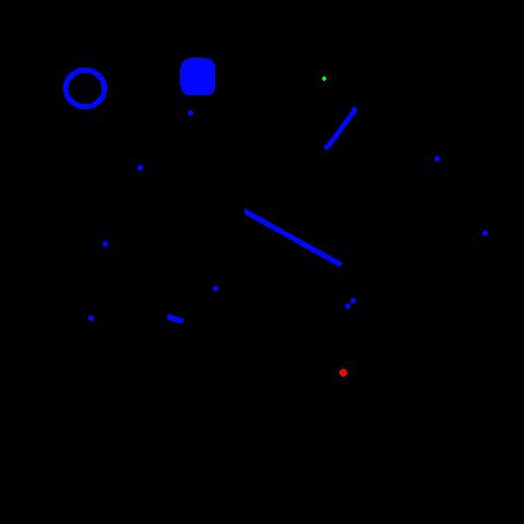
Sample Obstacle Field (obstacles in blue, start is green dot, goal
is red dot)
The program flips the robot image along both the x and y axes and
then traces the obstacles to produce the buffer zones. These are
shown in magenta when the program is running (pure blue + pure red).
With the two robots chosen (drawn in yellow when the program runs),
the center of the robot is fairly easy to estimate. That is the point
that cannot touch the magenta.
Potential Field:
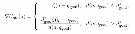
I implemented an attractive/repulsive
potential field. For the attractive gradient I used a combine
quadratic-linear attraction. Thus if the robot was further away than
a fixed value (5 meters in my case) it had a constant gradient
towards the goal. If the robot was closer than 5 meters, the
potential was quadratic with respect to the distance to the goal, so
the gradient was linear.
This is the potential function

This is the potential gradient
The repulsive potential from an obstacle is calculated with

Unfortunately since my program takes in discretized obstacles, it is
often hard to decide what is or isn't part of the same obstacle without
serious computation. Therefore my program actually counts each pixel of
an obstacle as a seperate obstacle, and thus ends up with the gradient
coming from a uniform distribution over the whole obstacle when the
summation of each repulsion vector is taken.
This means that a very small scalar is needed for the repulsive force.
or else the robot will fly away from obstacles faster than should be
possible. If the robot is at an area with a gradient of 0, it checks if
it is at the goal. If it is, it turns green, if not it turns red (local
minima).
The tuning factors of the robot were just the constants in these equations:
The attractive scalar ? (Ended up being around 3. Simply how much the goal attracts the robot)
The attractive distance threshold d* (where the attractive potential switches from quadratic to linear)
The repulsive scalar ? (became very small (0.0000001-ish)
The repulsive distance threshold Q* (effectively the sensor range
of the robot. Was around 10 meters since the robot itself is around 3
meters wide)
I changed the shape of the robot between the two worlds to show how the
obstacle buffers change. Successful
navigation
Failed
navigation