
Stephen Tully
Homework #2
16-735 Robotic Motion Planning
Instructor: Howie Choset
Tangent Bug Implementation in Matlab:
For this homework assignment, I implemented the Tangent Bug algorithm. I simulated a 3 degree-of-freedom mobile robot in a 2-dimensional workspace using Matlab.
The tangent bug algorithm:
While the robot is in the motion-to-goal state, the robot must look for intervals of connectivity in its range sensor array. The raw distance function can be stated:
This means that for each angle theta in the sensor array, the distance is equal to the distance to the closest obstacle (in that corresponging direction). In addition to this formulation, it should be noted that the distance function should be set to Infinity if an obstacle is not sensed for a given angle theta (due to limited sensor range). A visual representation of the distances measured (along with the intervals of connectivity spanning the dark endpoints) can be seen below:
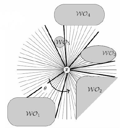
After encountering obstacles within the sensor range, the robot can detect disconinuity points in the raw distance function, which we call Oi. The robot simply chooses the best Oi for a given timestep and drives towards it:
![]()
The robot must keep track of this added distance value though. If it ever increases, the algorithm tells the robot to switch states (specifically boundary following). When boundary following, the robot drives along the tangent of the boundary. The robot keeps track of the distance, dfollowing, which is the closest sensed boundary distance to the goal, and dreach, the closest distance to the nearest obstacle in the direction of the goal.
If dreach ever falls below dfollowing, the robot can reenter the motion-to-goal state. This procedure is iterated on until the robot reaches the goal state. In some cases, the robot will completely loop around the boundary of an obstacle. Because the robot has knowledge about its position, it can detect cycles and automatically report a failure.
Implementation and Video Demos:
When viewing the demo videos, please note that the obstacles are represented by a series of line segments (to simulate an obstacle with a curved surface, I would simply use many line segments). Also, the robot is represented by a green arrow and the goal is represented by a red flag. The limiting sensor range of the robot is shown with a dotted circle drawn at the boundary of the sensing limit.
I used a simple model to drive the robot for a given input. The input was always determined using the tangent bug algorithm described above.
Above is a video of the robot performing a simple start-to-finish path while avoiding one obstacle. As you can see, the robot beings driving straight towards the goal because it does not encounter any obstacles. In a short while, the robot detects an obstacle and immediately finds the discontinuities in the raw distance function (represented by blue circles). The robot then drives towards the discontinuity point that best satisfies the distance metric outlined in the algorithm until it no longer has an obstacle blocking its way. It is complete when the robot successfully drives to the goal.

The video shown above is an example of when the tangent bug algorithm fails to reach the goal state. This is permissible because the tangent bug can detect when failure has occured. In this case, the goal position lies within an obstacle. The robot drives towards the obstacle, enters the boundary following state, but then never transitions to the motion-to-goal state. This is because the robot can never find either a close obstacle or a clear path to the goal (dreach cannot fall below dfollow). The robot successfully detects the failure when the boundary of the obstacle has been completely traversed, and then reports the failure.
Why I chose Tangent Bug:
I thought the tangent bug algorithm would perform better than the other, more simple, bug algorithms. It seems to generally be a more intelligent solution to the problem and for many cases takes a shorter path than the other bug implementations. Also, I just felt like implementing what I thought would be more challenging.
Additional Videos:
The following videos show more examples of the tangent bug algorithm successfully reaching the goal state. In both, the robot temporarily follows a boundary until the distance criterion is satisfied. The robot leaves the obstacle and either drives straight for the goal (last video) or encounters an additional obstacle (following video).
I would like to acknowledge Prof. Howie Choset for providing several of the images:
http://voronoi.sbp.ri.cmu.edu/~motion/lecture/lec3.pdf