Introduction
The search of optimal policy for a robot with many DOF is computationally hard task, due to the fact that for a control task spanning any interesting duration there are many possible trajectories have to be considered. One way to reduce this search task is to divide the search task into top-level footstep planner and lower level in-between footstep trajectory planner. One could imagine these algorithms as two interacting agents, advising each other on the cost/feasibility of the planning action. In the project I will investigate the possible ways that in-between trajectory planner could communicate the cost/feasibility of local trajectory to a top-level footstep planner for walking locomotion of a quadruped robot Little Dog.Approach
We consider that the global trajectory is specified as footstep location by a footstep planner and center of mass (COM) positions at the knot points (corresponding to each stance). The local policy optimizer will search for a control policy that will optimize the robot's motion for each step of the walk with respect to such metrics as
- velocity,
- stability of motion,
- smoothness of the motion.
Kinematic modeling
Kinematics
The robot has 4 legs each of which has 3 actuators, Figure 1. The legs inverse kinematics allows for 2 positions of the knee joint: backwards and forwards. For simplicity the trajectories that we consider in the project do not assume a switch betwene backward and forward knee positions.

Figure 1. Little Dog kinematics (adopted from the Little Doc manual, BDI).
Based on the LD manual and one-leg forward kinematics matlab code, I developed forwards kinematics and inverse kinematics subroutines in Matlab for the whole robot. For simplicity of the foot-ground contact modeling, I ignored the 1cm radius balls mounted on the feet.Simulation
A kinematic simulator is developed in Matlab based on the forward kinematics of the robot. The input to the simulator is:
- IDs of the 3 grounded feet.
- Joint angles.
Currently the following simplifying assumptions are made:
- The surface is flat
- The ground contact is a point
- There is no slippage

Figure 2. Little Dog simulation with support triangle (black) and the projection of the geometric center of the body (black circle).
Stability of a trajectory
Supporting pyramid
Consider static stability conditions for the robot. It states that the center of mass (COM) should be within the supporting polygon (triangle or quadrilateral in the case of the quadruped robot). In industry, there is also a notion of a pyramid, which we will call a supporting pyramid, within which the COM should be to ensure static stability given the range of perturbations, for example given a range of initial velocity. The intuitive notion is that to prevent tipping over the horizontal line AB, the COM should be under a plane crossing the horizontal surface via line AB and at a certain angle α. For a supporting triangle ABC, the permitted region that avoids tipping over each side of ABC will be a tetrahedron (pyramid) such that each non-horizontal face forms the same angle with the horziontal face. All other things equal, the less angle α, the shorter is the pyramid and the more stable the robot is.
Although this notion of supporting pyramid is intuitive and no clear derivation of it has been found, I will adopt it for its simplicity of implementation. At the end of the report I will attempt to formally derive an analogous notion. For now, I will discuss the conveniences afforded by the notion of the supporting pyramid for implementation.
Implementation: geometric properties
It's not difficult to see that the top vertex E of the supporting pyramid ABCE is directly above the inscribed circle of the triangle ABC. This gives a rather fast method of finding coordinates of E, given that the barycentric coordinates of the inscribed circle are a : b : c, where a, b, and c are the length of the sides of the triangle ABC across respective vertices A, B, and C (see Wikipedia: incircle).
Stance changes and stability pyramids
In this work I will consider the two-step fragment of a trajectory, which starts with a 3-leg stance (FL, HL, HR are grounded, FR is just lifted from ground), ends with a 3-leg stance (FL, HL, FR are grounded, HR is just hits the ground), such that:
- FL and HL feet stay grounded
- FR and HR feet's positions change
- first, foot FR moves to its final position
- then there is a (possibly instanteneous) 4-leg stance
- and finally foot HR is moved to its final position.
The support pyramids for the initial and final stances look as shown in Figures 3 and 4.

Figure 3. Support pyramids for the change of stances involing FR and HR legs (top view). See detailed description in text.

Figure 4. Support pyramids for the change of stances involing FR and HR legs (side view). See detailed description in text.
 Video of the initial and final stance supporting pyramids.
One of the properties of the pyramids is that the foot that moves first should reach its destination (i.e. the stance should change) before COM leaves the initial pyramid (in the case when the COM moves out of both pyramids). Since pyramids are convex bodies, the most time is afforded for the first change of stance if the change happens on the face of the first pyramid. Similarly the most time will be afforded for the last change of stance if the change is done when COM is on the surface of the second pyramid. Therefore the points where COM exits/enters pyramids are the natural descriptors of the trajectories.
Points marked by crosses represent the entry or exit points for a 4-leg stance (trajectory lies outside of either pyramid) of a 3-segment trajectory. Points marked by circles represent the trajectories that do not leave one of the pyramids (no need for the 4-leg stance of a non-zero duration), or 2-segment trajectories.
The examples of a 3-segment and 2-segment trajectories are shown in Figures 5 and 6.

Figure 5. A 3-segment trajectory (with a non-zero duration 4-leg stance middle segment).
Video of the 3-segment trajectory.
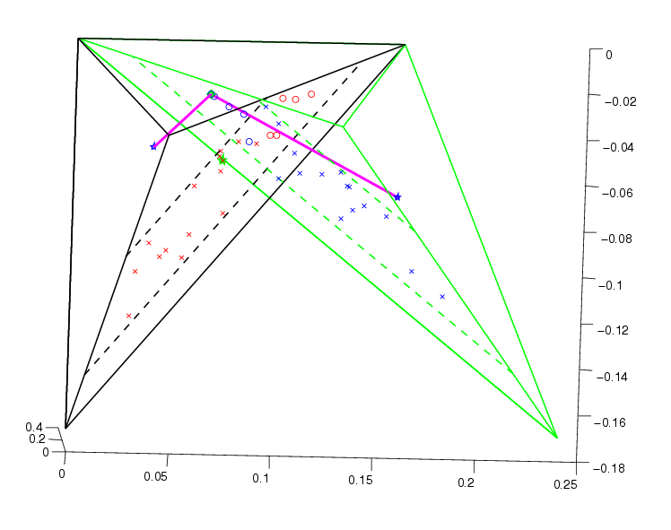
Figure 6. A 2-segment trajectory (without a non-zero duration 4-leg stance middle segment).
Video of the 2-segment trajectory.
Implementation: barycentric coordinates
Given that we would like to perform random sampling from a face of a pyramid, arguably the computational easiest way to do this is using barycentric coordinates (external link). Basically, in barycentric coordinates, the coordinates inside the stripe on the face of the pyramid are all those for which the coordinate corresponding to the top of the pyramid is within certain region e1,e2 and the other coordinates vary between 0 and 1. Uniform sampling from this strip on a simplex can be performed by sampling barycentric coordinates according to a Dirichlet distribution. Currently we perform a random sampling in uniform barycentric coordinates, for simplicity.
Cost function
A variety of cost functions could be implemented. For the current class of trajectories (piecewise linear with constant speed within each segment) I have chosen to simply compute cost as the sum of the squared velocities of the joint actuators. Since there are at most only 2 points of disconiuity of the acceleration, this cost function may also be reflective of the cost of smoothened trajectories around the respective piecewise linear seeds.
The costs of the 3-stance trajectory above is close to the cost of the 2-stance trajectory (0.1026 and 0.1029 respectively) despite the significant qualitative differences.
below are the videos of the robot following each of these trajectories.
Video of the robot following the 3-segment trajectory.
Video of the robot following the 2-segment trajectory.
Estimating the minimal-cost function in the vicinity of the original knot points
Can the local trajectory planner be helpful to the top-level footstep planner? What kind of interactions between these planners help improve the overall trajectories?
One way the local trajectory planner could give "advise" to the top-level footstep planner is by estimating the minimum cost functions around the proposed not points, in case a dramatic reduction of cost possible by relatively small "wiggle" of a knot point.
In this part I randomly sample the final COM position with expected distance from the original COM 1cm and standard deviation 1cm according to Gaussian distribution on the distance and a simple spherical coordinate-wise uniform distribution on the direction (Figure 7). After only 4 iterations of sampling the final positions (blue diamonds) a cheaper trajectory is found with its final position (red diamond) in the vicity of the original one (blue star).

Figure 7. Estimating the cost function in the viciting of the original COM knot point (details in text).
Derivation of an analogous stability creterion
Above we investigated the trajectory planning using the intuitive notion of the stability pyramids. We now will derive the relation on the angle α between the normal from the point mass m to the axis of rotation AB and the horizontal plane.
Consider the following sitation: the joints got locked as the robot was moving with velocity v towards the side AB of the supporting triangle ABC. What is the relation between the robots height h, angle α define above and the velocity v that ensure that the robot will not tip over the axis AB?
At the moment when joints got locked, the robot’s kinetic energy equals to its
rotational kinetic energy around the axis AB, which treating the robot as a point mass equals to Ek =  I
I 2 =
2 =  mr2
mr2 2, where m is the
mass of the robot, r is the radius of rotation (distance from COM to AB), and
2, where m is the
mass of the robot, r is the radius of rotation (distance from COM to AB), and
 is its angular velocity. Let h = r sinα is the initial height of the robot,
vt =
is its angular velocity. Let h = r sinα is the initial height of the robot,
vt =  r is the tangential velocity around axis AB, then the total kinetic energy
equals
r is the tangential velocity around axis AB, then the total kinetic energy
equals
 | (1) |
The robot will not tip over AB if its velocity equals 0 at the top of the trajectory, right above AB. At that instance the robot’s total energy will be its potential energy
 | (2) |
Equating (1) and (2) we obtain:
 | (3) |
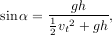
that is as long as sinα <  , the locking of the joints will not cause tipping
over the side of a supporting polygon.
, the locking of the joints will not cause tipping
over the side of a supporting polygon.
Since this relation is not as visual as the notion of stability pyramid, it is not immidiately clear how to generate trajectories that satisfy this critera from the beginning, instead of checking the compliance with the criteria afterwards. This could be a topic of future work.
Conclusion
In this work I have explored the possible interaction between the high-level footstep planner and the low-level trajectory optimizer for Little Dog. Based on an intuitive but informal notion of support pyramids a technique for sampling from a class of piecewise linear trajectories that are consistent with the stability criterion was developed and implemented. The results have shown that for the cost function (sum of squares of joint velocities) the optimal trajectory is not the shortest path connecting initial and final COM positions. Moreover, qualitatively different 2-segment and 3-segment trajectories are found that have close to optimal (so far found) cost. By sampling from a vicinity of the desired final COM position the low-level planner estimate the optimal-cost function around that point and give feedback to the high-level planner on possible modification of the top-level trajectory (footstep and COM knot point positions). Finally, I attempted to derive a formal criterion for static stability with initial velocity (that's it, given an initial velocity and locked joints, what are the conditions when the robot will not tip over a side of the supporting polygon). The derived relation is not as geometrically intuitive as supporting pyramids so its utility for generating the trajectories (as opposed to checking already generated trajectories against it) is not immidiately clear.Future work
- Other cost functions
- Smooth trajectories
- Other stability criteria, for example the derived one.
A little more distant future work
Incorporating dynamics and friction:
Explore hybrid wheel-legged locomotion: