
![]()

Appearance-Based Place Recognition
for Topological Localization
Iwan
Ulrich, Illah Nourbakhsh
Carnegie Mellon University - Robotics
Institute
Mobile Robot Programming
Laboratory
This web page gives a short overview of our novel appearance-based place recognition system for topological localization. The concept of topological localization was pioneered by Benjamin Kuipers in the late seventies. Topological localization algorithms are based on adjacency maps. Nodes represent locations, while arcs represent the adjacency relationships between the locations.
The main challenge of topological localization consists of reliably performing place recognition. An ideal sensor for this task is an omnidirectional color camera, because it provides rich information about the environment and does not suffer as much from perceptual aliasing as do most other sensors. The information contained in a single panoramic color image is in most cases sufficient to reliably recognize a location.
In short, our algorithm works as follows. In the mapping stage, we manually create an adjacency map of the environment. Creating such maps takes little time as no geometric information is required. In the learning stage, we acquire a series of representative reference images for each location. In the localization stage, the algorithm simply determines which reference image matches the current input image most closely.
|
|
|
Unfortunately, such an approach would require a lot of memory and would be difficult to implement in real-time. Inspired by the fields of image retrieval and object recognition, we replace the color images with their color histograms. Color histograms require little memory and histogram matching is a much faster process than image matching. In addition, image histograms are invariant to rotation of the image, which is especially attractive when combined with a panoramic vision system. For a given position, we therefore only need a single reference image, independent of the camera orientation.
 |
|
|
The resulting algorithm consist of the following four steps:
| 1) | Determine candidate locations based on current belief of robots location. | |
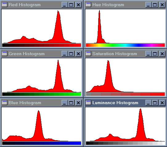
| 2) | Transform RGB input image into six 1-dimensional histograms: RGB and HLS. | |
| 3) | For each candidate location and each color band, determine the reference histogram that matches the input histogram most closely using the Jeffrey divergence as the dissimilarity metric. | |
| 4) | Combine the votes using an unanimous voting scheme. The resulting classification is either confident, uncertain, or confused. |
|
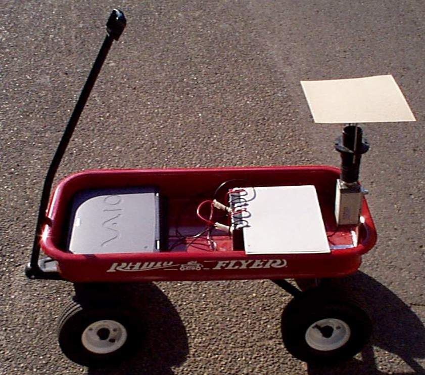
For experimental verification, we implemented our
passive localization algorithm on an all-terrain Radio Flyer wagon. Inside
the wagon are a laptop computer, batteries, and a color camera with an
omnicam. Using this platform, we evaluated our algorithm in four different
environments, three indoors and one outdoors. We pulled the wagon twice
through each environment, thus capturing two image sequences. We then used
the first image sequence as the reference images, and tested our algorithm with
the second sequence. Then switching the two sequences, we repeated the
test, thus getting two results for each environment. |
 |
Our first test was in an apartment with eight rooms. The
rooms of the apartment are very heterogeneous in appearance, and we thus
expected our algorithm to perform well in this environment. However, whenever
the robot believes that it is in the hallway, the system needs to differentiate
between seven rooms. As we had hoped, it turned out that our color histogram
representation is sufficiently expressive to distinguish between all these
rooms.
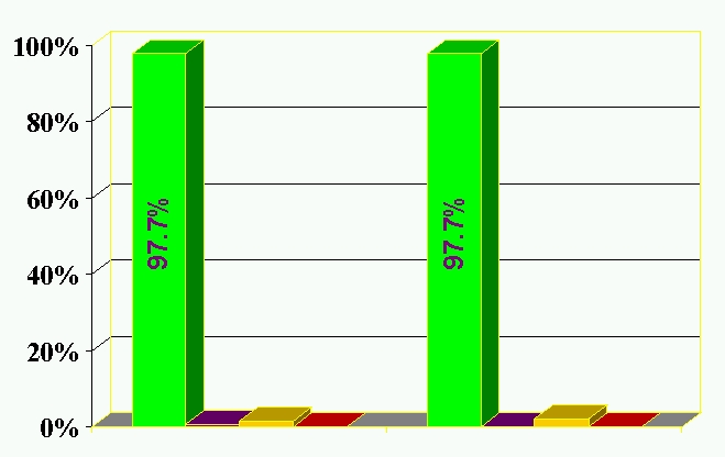
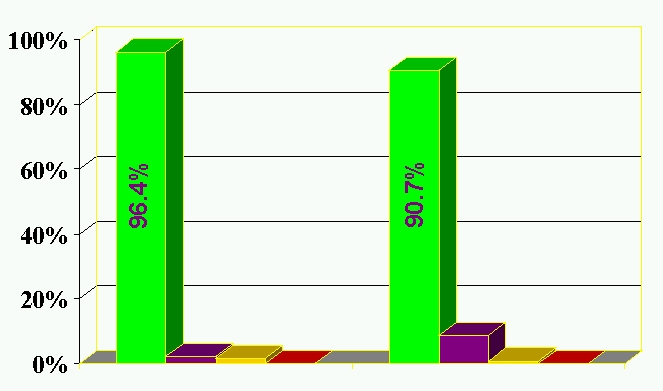
The graph shows the results for the two tests. The green bars show the correct
confident classification rates, which are in both cases very high, equal to
97.7%. The uncertain classification rates are shown in purple, and the confused
classification rates are shown in yellow. The red bars show the incorrect
confident classification rates, which were zero throughout all our experiments.
Because the confident classification rates were much higher than the rates of
uncertain and confused classifications, the system had no trouble tracking the
robot's position in both tests.
|
|
 |
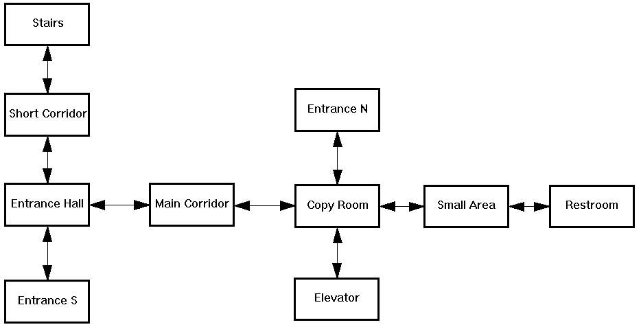
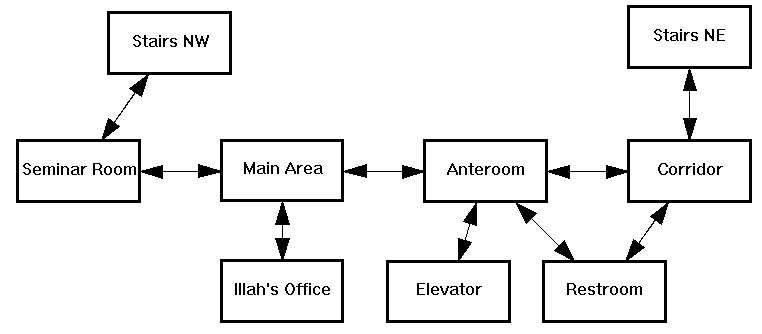
Next, we were wondering how our algorithm would perform in a
more homogeneous environment. So, we made two tests in Smith Hall, an office
building at CMU,
one on the first floor and one on the second floor. The first floor is rather
homogeneous in appearance, consisting mainly of corridors. The second floor is
more colorful, but it has a large open area, and we were curious if our
algorithm was able to deal with this situation.
Again, our algorithm performed well in all four tests. In our worst test, the
confident classification rate was 87.5%, which was still sufficient for the
system to successfully keep track of the robots position.
 |
|
 |
 |
|
 |
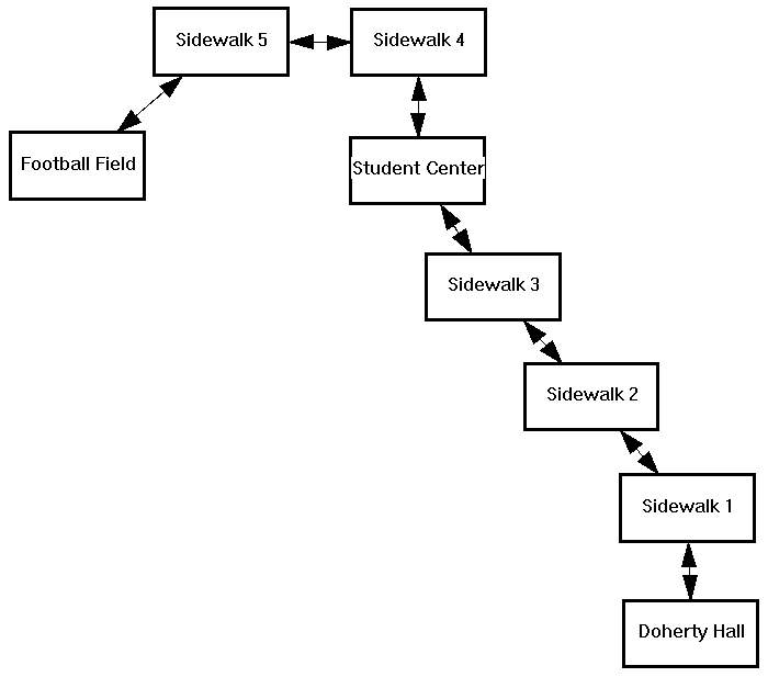
So, how well does our algorithm perform outdoors? The answer to this question was very important to us, because our initial motivation was to develop an algorithm that has actually the potential of working both indoors and outdoors. We tested our algorithm on a route that leads from Doherty Hall to the Football Field, which is a distance of about 250 meters. While the adjacency map was a little harder to define, the place recognition module performed very well, with correct confident classification rates of more than 90% in both tests.
 |
|
 |
In summary, our algorithm has a couple of appealing features. First, it performs well in a variety of environments, indoors as well as outdoors. There is no need to modify the environment. The adjacency maps can be built easily, as the environment does not need to be measured precisely. The algorithm is simple, performs in real-time, and is robust to small changes in the environment. And finally, the algorithm does not rely on odometry information at all, and is thus not affected by errors in odometry
For future work, we intend to improve our algorithm in two aspects. First, because our system is based on appearance, it is very sensitive to changes in the color distribution of the illumination. We hope that we will be able to implement a relatively simple color constancy algorithm by placing a reference chart with known reflectance properties into the cameras visual field. Second, the ideal localization system will be capable of creating topological maps on its own. Such a system would obviously be very user-friendly, and by allowing the system to define its own locations, we also hope to obtain even better results. And finally, such a system would make it practical for each color band to have its own adjacency map.
Ulrich, I., and Nourbakhsh, I., Appearance-Based Place Recognition for Topological Localization, IEEE International Conference on Robotics and Automation, San Francisco, CA, April 2000, pp. 1023-1029. Best Vision Paper Award.