Exploiting Internet Route Sharing for Large Scale Available Bandwidth Estimation
Ningning Hu, Peter Steenkiste
Carnegie Mellon University
{hnn, prs}@cs.cmu.edu
Abstract
Recent progress in active measurement techniques has made it possible to estimate end-to-end path available bandwidth. However, how to efficiently obtain available bandwidth information for the N2 paths in a large N-node system remains an open problem. While researchers have developed coordinate-based models that allow any node to quickly and accurately estimate latency in a scalable fashion, no such models exist for available bandwidth. In this paper we introduce BRoute - a scalable available bandwidth estimation system that is based on a route sharing model. The characteristics of BRoute are that its overhead is linear with the number of end nodes in the system, and that it requires only limited cooperation among end nodes. BRoute leverages the fact that most Internet bottlenecks are on path edges, and that edges are shared by many different paths. It uses AS-level source and sink trees to characterize and infer path-edge sharing in a scalable fashion. In this paper, we describe the BRoute architecture and evaluate the performance of its components. Initial experiments show that BRoute can infer path edges with an accuracy of over 80%. In a small case study on Planetlab, 80% of the available bandwidth estimates obtained from BRoute are accurate within 50%.
Recent progress in measurement techniques has made it possible to estimate
path available bandwidth [11,21,18,17,23,25]. These tools have enhanced our understanding of Internet end-to-end performance, and can be used to improve the performance of network applications.
However, how to efficiently obtain available bandwidth information for the N2 paths in a large N-node system remains an open problem. At the same time, a scalable available bandwidth estimation system has many potential applications. For example, a large service provider may want to know the available bandwidth performance for all its customers; P2P systems may want to know the available bandwidth between all node-pairs so as to select the best overlay topology; or people may want to monitor the health of a large scale system or testbed, like Planetlab [4].
Researchers have been able to build scalable systems for Internet latency estimation by using synthetic coordinated systems to significantly reduce the number of required measurements [22,12].
Unfortunately, we do not have a similar concept for available bandwidth. Brute force solutions will not work either. The overhead to probe one path is at least around 100KB [25,17], so measuring all end-to-end paths in a 150-node system would already require over 2GB for just one snapshot. This approach clearly does not scale to a large number of nodes, let alone to the whole Internet. Another challenge is that most available bandwidth measurement tools need to run on both ends of a network path to conduct measurements. This complicates the deployment of the tools significantly.
In this paper, we propose a scalable available bandwidth estimation system-BRoute. Here "available bandwidth" refers to the residual bandwidth left on an end-to-end path; it is determined by the available bandwidth of the bottleneck link, i.e., the link with smallest residual bandwidth. The goal of BRoute is to estimate the available bandwidth for any node-pair in a large system, with limited measurement overhead and limited cooperation among end nodes. BRoute is based on two observations. First, Hu et.al. [16] have observed that over 86% of Internet bottlenecks are within 4 hops from end nodes, i.e., on path edges. This suggests that bandwidth information for path edges can be used to infer end-to-end available bandwidth with high probability. Moreover, links near the end nodes are often shared by many paths, thus providing the opportunity to limit measurement overhead. This leads to the two key challenges in BRoute: how to measure the available bandwidth of path edges and how to quickly determine which edges a path uses.
The primary contribution of this paper is the BRoute system architecture: we discuss in Section 2 how it leverages routing information to reduce available bandwidth estimation overhead. In Sections 4-6, we first use an extensive set of measurement to show that many Internet paths exhibit the properties that BRoute relies on, we then present an algorithm that uses AS-level source and sink tree information to infer network path edges, and we finally describe how we measure the available bandwidth near end nodes. We discuss related work and conclude in Sections 7 and 8.
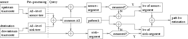
The BRoute design is based on two important observations. First, most bottlenecks are on path edges, so for most paths we only need to obtain available bandwidth information for both edges of a path to estimate path available bandwidth. Second, relatively few routes exist near the source and destination compared with the core of the Internet, thus simplifying the problem of determining which edges a path takes, and which bottleneck it encounters. These observations lead to the two main operations in BRoute. First, each node collects both routing and bottleneck information for the network "edge" to which it is attached, using traceroute and Pathneck [15], respectively. This information can be published, similar to a set of coordinates. Second, in order to estimate the available bandwidth between a source node and a sink node, any node can collect the routing and bottleneck information for the source and sink and use it to determine the route taken at the edges of the path, and thus the likely bottleneck location and available bandwidth.
Figure 1: End-segments and AS-level source/sink trees
Before we describe BRoute in more detail, let us first define what we mean by the "edge" of a path. It corresponds to the first E and the last N links of a complete IP level path; we will call these two partial paths the source-segment and sink-segment respectively. In this paper we will use E=4, N=4 since this captures most of the bottlenecks [16]. However, different values can be used. Formally, let the path from s to d be Path(s, d) = (r0 = s, r1, r2, ..., rn = d), here ri (1 ≤ i ≤ n−1) are routers on the path. Then the source-segment of Path(s, d) is srcSgmt(s, d) = (r0, r1, r2, r3, r4), and the sink-segment of Path(s, d) is sinkSgmt(d, s) = (rn−4, rn−3, rn−2, rn−1,rn). The left graph of Figure 1 illustrates the source-segments for end nodes a0, b0 and the sink-segments for end nodes c0, d0. The dashed lines indicate the omitted central part of the paths.
In this paper, we also use the term end-segment to indicate either a source-segment or a sink-segment.
If bottlenecks are on end-segments, we only need to consider the trees composed of the source-segments and sink-segments (called the source and sink tree), and we can ignore links within the "Internet Core" as illustrated in Figure 1. Each node can characterize both the structure and bandwidth properties of its source and sink tree. This information can be published in a central location or using a publish-subscribe system. Other nodes can then use that information to estimate the bandwidth for the paths toward or from that node. In large systems, many paths will share a same end-segment. For example, Path(a0, c0) and Path(b0, c0) share sink-segment (c8, c4, c2, c1, c0). This means that the measurement overhead is proportional to the number of end-segments, not the number of paths.
Based on the data set discussed in Section 3, we found that, assuming source/sink trees with a depth of 4, Internet end nodes have on average only about 10 end-segments, so the overhead is linear in the number of system nodes.
Besides identifying source and sink threes, BRoute needs to identify the source-segment and sink-segment for a path without direct measurement, i.e. identifying the leaves of the trees in Figure 1. BRoute does this using AS-level path information. Intuitively, for a pair of nodes s and d, if we know all the upstream AS paths from s (called the AS-level source tree or srcTree(s)) and all the downstream AS paths toward d (called the AS-level sink tree or sinkTree(d)), then Path(s, d) should pass one of their shared ASes. For example, the right graph of Figure 1 illustrates the upstream AS paths from a0, and the downstream AS paths toward c0. Assume that A7 is the only shared AS then this means that path Path(a0, c0) must pass through A7, and we can use A7 to identify srcSgmt(a0, c0) and sinkSgmt(c0, a0). We will call the AS that is shared and on the actual path the common-AS. Of course, there will typically be multiple shared ASes between srcTree(s) and sinkTree(d). We will discuss in Section 5.1 how to uniquely determine the common-AS.
The BRoute architecture includes three components: system nodes, traceroute landmarks, and an information exchange point. System nodes are Internet nodes for which we want to estimate available bandwidth; they are responsible for collecting their AS-level source/sink trees, and end-segment available bandwidth information. Traceroute landmarks are a set of nodes deployed in specific ASes; they are used by system nodes to build AS-level source/sink trees and to infer end-segments. An information exchange point, such as a server or publish-subscribe system, collects measurement data from system nodes and the bandwidth estimation operations can then be carried by either the server or alternatively, by the querying client. For simplicity, we will assume the use of a BRoute server in this paper.
Figure 2: BRoute System Architecture
BRoute leverages two existing techniques: bottleneck detection [15] and AS relationship inference [14,26]. Bottleneck detection is used to measure end-segment bandwidth, and AS relationship information is used to infer the end-segments of a path. The operation of BRoute can be split into a pre-processing stage and a query stage (Figure 2):
Pre-processing: In this stage, each system node conducts a set of traceroute measurements to the traceroute landmarks. Similarly, traceroute landmarks conduct traceroutes toward system nodes. The system node then uses the traceroute information to construct AS-level source and sink trees. Next the system node identifies its source-segments and sink-segments and uses Pathneck to collect bandwidth information for each end-segment.
This information is reported to the BRoute server.
Query: Any node can query BRoute server for an estimate of the available bandwidth between two system nodes-s to d. The BRoute server will first identify the common-AS between srcTree(s) and sinkTree(d). The common-AS is used to identify the end-segments srcSgmt(s, d) and sinkSgmt(d, s) of Path(s, d), and the BRoute server then returns the smaller of the available bandwidths for srcSgmt(s, d) and sinkSgmt(d, s) as the response to the query.
A distinguishing characteristic of BRoute is that it uses AS-level source/sink tree computation to replace expensive network measurements. In the following four sections, we first describe the data sets used in our analysis, and we then elaborate on three central features of BRoute: key properties of AS-level source and sink trees, end-segment inference, and end-segment bandwidth measurement.
The evaluation of the BRoute design uses five data sets:
The BGP data set
includes BGP routing tables downloaded from the following sites on 01/04/2005: University of Oregon Route Views Project [8], RIPE RIS (Routing Information Service) Project [5],
and the public route servers listed on [7]. These BGP tables include views from 190 vantage points, which allow us to conduct a relatively general study of AS-level source/sink tree properties.
The Rocketfuel data set is mainly used for IP-level analysis of end-segments. We use the traceroute data collected on 12/20/2002 by the Rocketfuel project [24,6], where 30 Planetlab nodes are used to probe over 120K destinations.
The Planetlab data set was collected by the authors using 160 Planetlab nodes at different sites. It includes traceroute result from each node to all the other nodes and it is used to characterize AS-level sink tree properties.
The AS-Hierarchy data set was downloaded from [1] to match our route data sets. It contains two snapshots: one from 01/09/2003 (the closest available data set to the Rocketfuel data set in terms of measurement time), which is used for mapping Rocketfuel data set; the other from 02/10/2004, which is the latest snapshot available, and is used for mapping BGP and Planetlab data sets. This data set uses the heuristic proposed by Subramanian et.al. [26] to rank all the ASes in the BGP tables used in the computation.
The IP-to-AS data set was downloaded from [3]. Its IP-to-AS mapping is obtained using a dynamic algorithm, which is shown to be better than results obtained directly from BGP tables [20].
The definition of AS-level trees is based on the ranking system from [26], where all ASes are classified into five tiers. Tier-1 includes ASes belonging to global ISPs, while tier-5 includes ASes from local ISPs. Intuitively, if two connected ASes belong to different tiers, they should have a provider-to-customer or customer-to-provider relationship; otherwise, they should have a peering or sibling relationship. To be consistent with the valley-free rule [14], we say that an AS with a smaller (larger) tier number is in a higher (lower) tier than an AS with a larger (smaller) tier number. An end-to-end path needs to first go uphill from low-tier ASes to high-tier ASes, then downhill until reaching the destination (see Figure 3).
Formally, let Tier(ui) denote the tier number of AS ui, then an AS path (u0, u1, ..., un) is said to be valley-free iff there exist i, j (0 ≤ i ≤ j ≤ n) satisfying:
The maximal uphill path is then (u0, u1, ..., uj), and the maximal downhill path is (ui, ui+1, ..., un). The AS(es) in the highest tier {ui, ..., uj} are called top-AS(es).
We can now define the AS-level source tree for a node s as the graph srcTree(s) = (V, E), where V = {ui} includes all the ASes that appear in one of the maximal uphill paths starting from s, and E = {(ui, uj) | ui ∈ V, uj ∈ V} includes the directional links among the ASes in V, i.e. (ui, uj) ∈ E iff it appears in one of the maximal uphill paths starting from s. The AS-level sink tree is defined similarly, except that we use maximal downhill paths.
In this subsection, we show that AS-level source/sink trees closely approximate tree structures. As we will see in the next section, this is important, since it allows BRoute to map the common-AS to a unique tree branch. There are two reasons why an AS-level source/sink tree may not be a tree. First, ASes in the same tier can have a peering or a sibling relationship, where data can flow in either direction; that can result in a loop in the AS-level source/sink tree. Second, customer-to-provider or provider-to-customer relationship can cross multiple tiers.
To study how closely AS-level source/sink trees approximate real tree structures, we define the tree-proximity metric. For AS-level source trees it is defined as follows; the definition for AS-level sink trees is similar.
We first extract all maximal uphill paths from a data set that provides path information, for example, as obtained from BGP (BGP data set) or traceroute (Rocketfuel data set). This is done for each view point, where a view point is either a peering point (BGP data set) or a measurement source node (Rocketfuel data set). We then count the number of prefixes covered by each maximal uphill path, and use that number as the popularity measure of the corresponding maximal uphill path. Next we construct a tree by adding the maximal uphill paths sequentially, starting from the most popular one. If adding a new maximal uphill path introduces non-tree links, i.e., gives a node a second parent, we discard that maximal uphill path. As a result, the prefixes covered by that discarded maximal uphill path will not be covered by the resulting tree. The tree proximity of the corresponding AS-level source tree is defined as the percentage of prefixes covered by the resulting tree. While this greedy method does not guarantee that we cover the largest number of prefixes, we believe it provides a reasonable estimate on how well an AS-level source tree approximates a real tree.
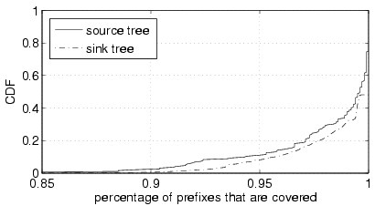
Figure 4: The tree proximities of the AS-level source/sink trees from the BGP
data set
Using the BGP data set, we can build an AS-level source tree for each of the 190 view points. The distribution of the tree proximities is shown as the solid curve in Figure 4. About 90% of the trees have a proximity over 0.95, and over 99% are above 0.88. This shows that the AS-level source trees indeed resemble real trees. This conclusion is consistent with the finding by Battista et.al. [9], who noticed that a set of AS relationships can be found to perfectly match the partial view of BGP routes from a single vantage point.
We also built AS-level sink trees using the BGP data set. We identified 87,877 prefixes that are covered by at least 150 view points, i.e., for which we can get over 150 maximal downhill paths. We picked the number "150" because it can give us a large number of trees.
The results, illustrated by the dot-dash curve in Figure 4, are very similar with those for AS-level source trees. Actually, the tree-proximity from sink trees are slightly better, which could be a result of the limited number of downstream routes used for the AS-level sink-tree construction.
We repeated the same analysis for the Rocketfuel data set and reached similar conclusions. When looking at the causes for discarding a maximum uphill path during tree construction, we found that the second cause for violations of the tree property, i.e. the creation of multiple paths to reach a higher tier AS, was by far the most common reason. We speculate that these violations are caused by load-balancing-related routing policies such as MOAS (Multiple Origin AS) and SA (Selected Announced Prefixes).
As a final note, we also looked at how to efficiently measure AS-level source/sink tree. We found that if we deploy one landmark in each of the tier-1 and tier-2 ASes (totally 237 ASes in the 02/10/2004 AS-Hierarchy data set), we can cover at least 90% of most AS-level source/sink trees. That suggests that 200-300 landmarks can do a reasonable job.
We are now ready to describe two key operations of BRoute:
how to pick the common-AS, and how to use the common-AS to identify the
source-segment and sink-segment of a path.
Algorithm:
Typically, an AS-level source tree and an AS-level sink tree share multiple ASes. We use the following algorithm to choose one of them as the common-AS. Based on the fact that most AS-level routes follow the shortest AS path [19], the algorithm first searches for the shared ASes that are closest to the root ASes in both srcTree(s) and sinkTree(d). If we are left with multiple candidates, we pick the one that has the highest probability to appear on Path(s, d) in the measurement. We must also consider two special cases: (a) one or both root ASes can be shared, and (b) there may be no shared AS between the measured trees. For case (a), we return either one or both root ASes as the common-AS(es), while for case (b), we consider all ASes as shared, and we pick based on their occurrence probabilities.
Evaluation:
Given the data we have, we can use two methods to evaluate the above algorithm. The first is to apply the algorithm on the AS-level source and sink trees described in Section 4.2. This method is straightforward and is used in the case study of BRoute discussed in Section 6. This method however has the drawback that it is based on limited downstream data, so the AS-level sink trees can be incomplete. In this section we use a different method: we evaluate the algorithm using the srcTree(d) to replace the incomplete sinkTree(d). The basis for this method is the observation that the AS-level trees are only used to determine the end-segments of a path (we do not need the AS-level path itself), and the AS-level source tree may be a good enough approximation of the AS-level sink tree for this restricted goal. This in fact turns out to be the case in our data sets.
Using the BGP data set, we construct an AS-level source tree for each vantage point, infer the common-AS for each pair of vantage points, and then compare the result with the actual AS paths in the BGP tables. To make sure we have the correct path, we exclude those AS paths whose last AS is not the AS of the destination vantage point. For the 15,383 valid AS paths, the common-AS algorithm selects the wrong common-AS for only 514 paths, i.e. the success rate is 97%. Furthermore, for the 14,869 correctly inferred common-ASes, only 15 are not top AS, which confirms our intuition that the common-AS inferred is typically a top-AS, where the maximal uphill and downhill paths meet.
Given that the AS-level source and sink trees closely follow a tree structure,
the common-AS can be easily used to identify a unique branch in both the
AS-level source and sink tree. We now look at how well this AS-level tree branch can be used to determine IP-level end-segments of the path.
Ideally, for any AS A ∈ srcTree(s), we would like to see that all upstream paths from s that pass A share the same source-segment e. If this is the case, we say A is mapped onto e, and every time A is identified as the common-AS, we know that the source-segment of the path is e. In practice, upstream paths from s that pass A could go through different source-segments, due to reasons such as load-balance routing or multihoming. To quantify the differences among the source-segments that an AS can map onto, we define the coverage of source-segments as follows. Suppose AS A is mapped to k (k ≥ 1) source-segments e1, e2, ..., ek, each of which covers n(ei) (1 ≤ i ≤ k) paths that pass A. The coverage of ei is then defined as n(ei) / ∑i=1k n(ei). If we have n(e1) > n(e2) > ... > n(ek), then e1 is called the top-1 source-segment, e1 and e2 are called the top-2 source-segments, etc. In BRoute, we use 0.9 as our target coverage, i.e., if the top-1 source-segment e1 has coverage over 0.9, we say A is mapped onto e1.
We use the Rocketfuel data set to analyze how many end-segments are needed to achieve 0.9 coverage. The 30 AS-level source trees built from this data set include 1687 ASes (the same AS in two different trees is counted twice), 1101 of which are mapped onto a single source-segment (i.e. coverage of 1). Among the other 586 ASes (from 17 trees) that are mapped onto multiple source-segments, 348 can be covered using the top-1 source-segments, so in total, (1101 + 348 = 1449) (85%) ASes can be mapped onto a unique source-segment. If we allow an AS to be covered using the top-2 source-segments, this number increases to 98%, i.e., only 2% (17 ASes) cannot be covered.
We used the Planetlab data set, which includes many downstream routes for each node, to look at the sink-segment uniqueness. We found that the above conclusion for source-segments also applies to sink-segment. Among the 99 nodes that have at least 100 complete downstream routes, 69 (70%) nodes have at least 90% of the ASes in their AS-level sink tree mapped onto top-1 sink-segments, while 95 (96%) nodes have at least 90% of their ASes mapped onto top-2 sink-segments.
Based on these end-segment properties, we map the common-AS onto top-1 or top-2 end-segments. In the first case, we return the available bandwidth of the top-1 end-segment. In the second case, we return the average of the available bandwidth of the two top-2 end-segments as the path bandwidth estimate. This method will work well if the reason for having top-2 end-segments is load balancing, since the traffic load on both end-segments is likely to be similar.
BRoute uses Pathneck to measure end-segment bandwidth. Although Pathneck only provides available-bandwidth upper or lower bounds for links on the path, it also pinpoints the bottleneck location, so we know if the measured path bandwidth applies to the source-segment or sink-segment.
In BRoute, each node can easily use Pathneck to measure the available bandwidth bounds on its source-segments. However, to measure sink-segment bandwidth, system nodes need help from other nodes in the network.
BRoute can collect end-segment bandwidths in two modes: infrastructure mode and peer-to-peer mode. In the infrastructure mode, we use bandwidth landmarks that have high downstream bandwidth to measure the sink-segment bandwidth of system nodes. The bandwidth landmarks can use the same physical machines as the traceroute landmarks. In this mode, a system node uses its AS-level source tree to pick a subset of bandwidth landmarks. The system node will use Pathneck to measure source-segment bandwidth, using the selected bandwidth landmarks as destinations. Similarly, the bandwidth landmarks, at the request of the system, will measure the sink-segment bandwidth using the system node as Pathneck's destination. Clearly, each bandwidth landmark can only support a limited number of system nodes, but a back-of-envelop calculation shows that a bandwidth landmark with a dedicated Internet connection of 100Mbps can support at least 100K system nodes, assuming the default Pathneck configuration.
In the peer-to-peer mode, end-segment bandwidths are measured by system nodes themselves in a cooperative fashion. That is, each system node chooses a subset of other system nodes as peers to conduct Pathneck measurements, so as to cover all its end-segments.
We use a simple greedy heuristic to find the sampling set. The main idea is to always choose the path whose two end nodes have the largest number of un-measured end-segments. In the Planetlab data set, this algorithm finds a sampling set that includes only 7% of all paths, which shows it is indeed effective. The peer-to-peer mode scales well, but it needs to support node churn, which can be complicated. Also, some system nodes may not have sufficient downstream bandwidth to accurately measure the available bandwidth on sink-segments of other system nodes.
Based on the peer-to-peer mode, we conducted a case study of BRoute on Planetlab using the design of Figure 2. The results show that over 70% of paths have a common-AS inference accuracy over 0.9, and around 80% of paths have an available bandwidth inference error within 50%. Although not perfect, these results are encouraging considering that available bandwidth is a very dynamic metric.
BRoute is motivated by coordinate-based systems [22,12] used for delay inference,
but it does not explicitly construct a geometric space. BRoute instead leverages existing work on AS relationships [14,26] as described in Section 4.1. Recent work on AS relationships identification [9,19] could help improve BRoute.
For example, [19] shows how to infer the AS path for a pair of nodes using only access to the destination node.
AS-level source/sink trees are an important part of the BRoute design. Others have also identified such tree structure, but at the IP level. For example, Broido et.al. [10] pointed out that 55% of IP nodes in their data set are in trees. Recently, Donnet et.al. [13] propose the Doubletree algorithm, which uses an IP-level tree structure to reduce traceroute redundancy in IP-level topology discovery. Using our terminology, the Doubletree is a combination of a source-node IP-level source tree and a destination-node IP-level sink tree. In contrast, BRoute leverages AS-level tree and we quantify how closely they approximate real trees.
BRoute uses Pathneck [15] for bandwidth measurements since it also provides the bottleneck location. For different application requirements, other bandwidth measurement tools [11,21,18,17,23,25]
can be used. In a broad sense, BRoute is a large-scale measurement infrastructure that uses information sharing to estimate available bandwidth efficiently. Several measurement architectures have been proposed, but they typically focus on ease of deployment and of data gathering. A good survey can be found in [2].
In this paper, we presented the system architecture and primary operations of BRoute-a large-scale bandwidth estimation system. We explain we take advantage of Internet route sharing, captured as AS-level source/sink trees, to reduce bandwidth estimation overhead. We show that AS-level source/sink trees closely approximate a tree structure, and demonstrate how to use this AS-level information to infer end-segments, where most bottlenecks are located. In a small case study on Planetlab, 80% of the available bandwidth estimates obtained from BRoute are accurate within 50%.
Our BRoute study is only a first step towards a practical, scalable bandwidth estimation infrastructure. More work is needed in several areas.
First, larger scale measurement studies are need to evaluate and refine BRoute.
Second, we need to improve our understanding of several aspects of the algorithms, including end-segment inference, path available bandwidth estimation, and landmark selection.
Finally and perhaps most importantly, we would like to deploy BRoute, both as a public service and as a platform for ongoing evaluation and research.
Acknowledgements
This research was funded in part by NSF under award number CCR-0205266
and in part by KISA (Korea Information Security Agency) and CyLab Korea.
G. D. Battista, M. Patrignani, and M. Pizzonia.
Computing the types of the relationships between autonomous systems.
In Proc. IEEE INFOCOM, April 2003.
A. Broido and k. clafy.
Internet topology: Connectivity of ip graphs.
In Proc. SPIE International Symposium on Convergence of IT and
Communication, 2000.
R. Carter and M. Crovella.
Measuring bottleneck link speed in packet-switched networks.
Technical report, Boston University Computer Science Department,
March 1996.
N. Hu, L. Li, Z. Mao, P. Steenkiste, and J. Wang.
Locating Internet bottlenecks: Algorithms, measurements, and
implications.
In Proc. ACM SIGCOMM, August 2004.
N. Hu, O. Spatscheck, J. Wang, and P. Steenkiste.
Optimizing network performance in replicated hosting.
In The Tenth International Workshop on Web Caching and Content
Distribution (WCW 2005), September 2005.
N. Hu and P. Steenkiste.
Evaluation and characterization of available bandwidth probing
techniques.
IEEE JSAC Special Issue in Internet and WWW Measurement,
Mapping, and Modeling, 21(6), August 2003.
M. Jain and C. Dovrolis.
End-to-end available bandwidth: Measurement methodology, dynamics,
and relation with TCP throughput.
In Proc. ACM SIGCOMM, August 2002.
B. Melander, M. Bjorkman, and P. Gunningberg.
A new end-to-end probing and analysis method for estimating bandwidth
bottlenecks.
In Proc. IEEE GLOBECOM, November 2000.
V. Ribeiro, R. Riedi, R. Baraniuk, J. Navratil, and L. Cottrell.
pathchirp: Efficient available bandwidth estimation for network
paths.
In Proc. PAM, April 2003.
L. Subramanian, S. Agarwal, J. Rexford, and R. H. Katz.
Characterizing the Internet hierarchy from multiple vantage points.
In Proc. IEEE INFOCOM, June 2002.