Lecture 27: Scalable Algorithms and Systems for Learning, Inference, and Prediction
Notes for Lecture 27
Preliminaries
Two major challenges in real-world machine learning:
- Massive datasets: For example, Wikipedia, YouTube videos, Tweets etc.
- Massive models: Parameters in billions for complicated architectures like deep learning models, Bayesian architectures etc. Even simple models like regression can have a large number of parameters.
We need scalable ML algorithms to overcome these challenges. We wish to develop distributed ML algorithms whose performance scales almost linearly with the number of machines.
We can coarsely divide the machine learning methods into two types:
- Probabilistic programs: Markov Chain Monte Carlo methods, Variational Inference etc.
- Optimization programs: Like gradient descent and related algorithms
We see that ML algorithms have a property of being iterative-convergent. That is, incremental updates are made to the state of the model until the state is stationary. Another important property of such algorithms is the fact that unlike most traditional algorithms, where each step must be perfect to get the final output, since ML algorithms are essentially a search for a state over a space, a slight noise in the trajectories is well-tolerated. That is, these ML algorithms can self-heal. These are important properties that facilitate distributed machine learning. We can now formally define an ML program as a search for a $\theta^*$ such that:
where $\Omega$ is some regularization term and $\mathcal{L}$ is some function of the data and the parameters. A typical algorithm to find this $\theta^*$ looks like this:
for t from 1 to T:
  doSomething();
  updateParameters();
  doSomethingElse();
Where the updateParameters() function looks something like:
where $\Delta_f\theta(\mathcal{D})$ is an incremental update calculated as a function of the dataset and the previous value of the parameters. Since function scales with both the data and the parameters, it is typically the most computationally expensive portion of the entire algorithm and benefits from parallelization.
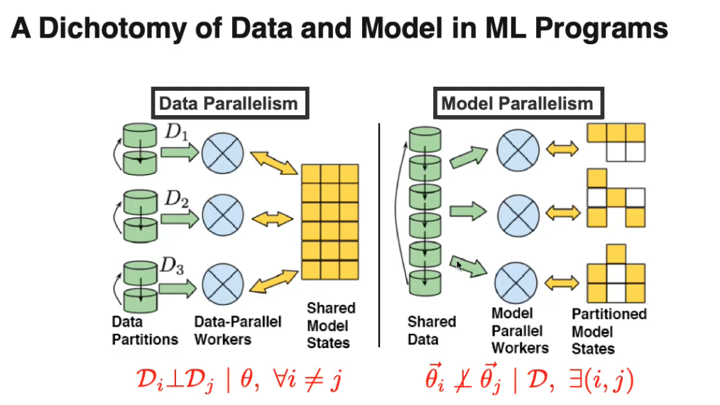
We can broadly categorize the parallelization techniques that we use into two categories:
- Data parallel methods: The data is divided into smaller chunks and sent to different machines, which calculate updates relevant to a particular chunk, after which some sort of an aggregation step is performed to combine the work done by different machines.
- Model parallel methods: The model parameters are divided into different sets and sent to different machines and each machine calculates the updates for those specific parameters.
Of course, a combination of these two approaches is also possible.
Parallelization for Optimization Algorithms
A concrete optimization problem: Linear Regression
Consider the case of a simple linear regression with a squared error loss. We wish to find:
Where $\Omega$ is a regularization term which may be used to induce sparsity, or incorporate domain knowledge. The form of $\Omega$ may vary depending on what the underlying priors are about the structure of the problem. This tells us that linear regression is actually a collection of models, where we can pick a data-fitting loss function and a regularization term and take a weighted sum of the two. Therefore, any parallel algorithms that one might come up with should be fairly general.
Recap: The sequential Stochastic Gradient Descent (SGD)
Consider the following optimization problem:
Vanilla gradient descent updates the parameters in the following manner:
Stochastic gradient descent uses a noisy estimate of the gradient using a single point:
This converges almost surely to the global optimum for convex problems. In practice, we actually use a batch of data points instead of a single one, which decreases the variance of the gradient and also allows us to use efficient matrix multiplication libraries.
Parallel Stochastic Gradient Descent (PSGD)
It is a data-parallel extension to the vanilla stochastic gradient descent, wherein you divide the dataset into chunks and send a chunk to one machine with a copy of the parameters. In PSGD, each machine runs SGD with its chunk of data till it converges. Finally the different versions of the parameters are aggregated, for example, by taking the mean of the parameters. One potential downside of the algorithm is that taking the mean of parameter copies that have individually converged to minimas need not necessarily mean that the resultant parameters lie in a minima.
Hogwild!: A lock-free approach to PSGD
Our goal is to optimize a function of the form, which is common in sparse models:
where $E$ is the set of indices of all the parameters, $e$ is a subset of these indices, $f_e$ is a function that operates only on the parameters which have their index in $e$ and $\theta_e$ is the set of parameters with their index in $e$. In such a case, we can use the Hogwild! algorithm as follows:
for each core in parallel:
  for i from 1 to T:
    Sample e uniformly at random from E
    Read current parameter set θ_e and calculate gradients for f_e
    Sample a single coordinate from θ_e
    Perform SGD on that single coordinate with a small step size
We can ignore memory-locking the parameters when computing the updates because the chances of collisions are very low.
This algorithm works very well for single machines with multiple processing units, but is less ideal for distributed systems due to the inherent delay in the communication between nodes. In particular, in case of uncontrolled delays in the communication between machines in lock-free environments, we face two issues:
- A high variance in the delay, which is typical of distributed systems, causes a slower convergence
- A higher delay increases the variance of the parameters, that is, causes instability during convergence
Parallel SGD with Key-Value
In this paradigm, we maintain a parameter server whose sole job is to maintain a master copy of the parameters and handle synchronization among the updates from the worker nodes, whose sole job is to calculate parameter updates and send to the server. There can be different synchronization schemes in place:
- Bulk synchronous parallel: In this scheme, all the worker nodes get a fresh copy of the parameters from the master, calculate the updates using these parameters and send the updates to the master. The master then waits till it has received an update from all the nodes and then updates the parameters. It then broadcasts the new parameters to all the nodes. This is slowed down by the fact that the nodes have to wait for all other nodes to finish to receive a new copy.
- Asynchronous parallel: Essentially Hogwild!. The worker nodes do their jobs without waiting for the slower nodes to catch up.
- Stale synchronous/bounded asynchronous parallel: A middle ground between bulk synchronous and asynchronous schemes. Unlike the bulk synchronous scheme, the worker nodes do not wait for all the other nodes to have calculated an update, but unlike the asynchronous scheme, they’re not allowed to get too far ahead of the slower nodes either. In particular, there is a limit (staleness threshold) to the number of steps a particular worker can be ahead by, after which it must wait for the slower threads to catch up.
Empirically, it has been shown that stale synchronous parallel updates converge faster (in seconds) than the other two.
Sequential Coordinate Descent
Another popular optimization technique that is commonly used is the Coordinate Descent Algorithm. It works as follows:
- Randomly pick a single parameter $\theta_i$ from the vector of parameters $\theta$
- Given the loss function $\mathcal{L}(\theta)$, solve the equation $\frac{\partial \mathcal{L}(\theta)}{\partial\theta_i} = 0$ and update the parameter $\theta_i$ to the solution
- Repeat
This algorithm suits Lasso regression very well as the partial derivative turns out to be a linear function of $\theta_i$, and therefore the equation is easily solvable.
Block Coordinate Descent:
Coordinate Descent lends itself to a simple extension called Block Coordinate Descent. Instead of picking a single parameter in the first step, we select a subset of parameters. In the second step, we solve a system of equations by obtained by setting the partial derivatives with respect to all the parameters in the subset to zero.
Shotgun, a Parallel Coordinate Descent Algorithm
It is an algorithm very similar to Hogwild!, in that it is simple to implement and forgoes “correctness” for simplicity. In this algorithm, each worker randomly picks a coordinate (a single parameter) to update. The updates are done in parallel with no locks. If the features are nearly independent, it scales almost linearly with the number of machines. However, as can be seen in the image below, concurrent updates to coordinates often overshoot if the features are correlated and may slow down the covergence, or in the worst case, cause a divergence.

Block-greedy Coordinate Descent
It is a generalization of the other paralllel coordinate descent algorithms. The coordinates (parameters) are divided into $B$ blocks such that the inter-block correlation is minimal. Each node picks a different block, and then picks a parameter from that block to update. Again, the updates are done without locks. This algorithm has a sublinear convergence. However, the downside is that dividing the parameters into uncorrelated blocks is difficult.
Parallel Coordinate Descent with Dynamic Scheduler
STRADS (STRucture-Aware Dynamic Scheduler) is a scheduler that allows dynamic scheduling of parameter updates in coordinate descent. It focuses on two things:
- Dependency checking: If two coordinates are correlated, do not compute them in parallel.
- Prioritization: Choose the coordinate to update with a probability proportional to its historic rate of change. Intuitively, a parameter that changes rapidly will probably cause a quicker decrease of the loss function.
These two things together can provide an order of magnitude increase in the rate of convergence.
Advanced Optimization for Complex Constraints: Proximal Gradient methods:
Projected Gradients:
Suppose we have an optimization problem:
where $f$ is some smooth function and C is a convex set of points. We can define a $0-\infty$ indicator function $\iota_C$ such that:
The optimization then reduces to:
An iterative solution can be obtained using the projected gradient descent algorithm. One iteration looks like:
- $v \leftarrow w - \eta\nabla f(w)$
- $w \leftarrow \arg\min_z \frac{1}{2\eta}\lVert v - z\rVert_2^2 + \iota_C(z) = \arg\min_{z \in C}\frac{1}{2\eta}\lVert v - z\rVert_2^2$
Intuitively, it is equivalent to taking an unconstrained step in the direction of the gradient, and then projecting the new position to the closest point in the feasible set.
Proximal Gradients:
Proximal gradients are a generalization of projected gradients, in which the indicator function $\iota_C$ is replaced by an arbitrary function $g(z)$, which may model constraints, regularizations etc. Intuitively, now, not only can we restrict $w$ to a feasible region, but can also say which regions are better than the others. Now one iteration of the algorithm looks like:
- $v \leftarrow w - \eta\nabla f(w)$
- $w \leftarrow \arg\min_z \frac{1}{2\eta}\lVert v - z\rVert_2^2 + g(z)$
The minimization problem in the second step has been well-studied, and closed form operators have been derived for the expression $\arg\min_z \frac{1}{2\eta}\lVert v - z\rVert_2^2 + g(v)$ for different $g$. We denote:
Also, for certain conditions derived by
Accelerated Proximal Gradients:
It has been proved that the covergence rate for PG is $O(1/\eta t)$. However, if we add a momentum term, as done in vanilla SGD optimizations, it improves to $O(1/\eta t^2)$. After incorporating the momentum term, the algorithm looks like:
- $v^t \leftarrow w^t - \eta\nabla f(w^t)$
- $u^t \leftarrow P^\eta_g(v^t)$
- $w^{t+1} \leftarrow u^t + \frac{t-1}{t+1}(u^t - u^{t-1})$
Parallel Accelerated Proximal Gradient Descent
Parallel (accelerated) PG is typically implemented using a parameter server in a bulk-synchronous fashion. The typical strategy goes as follows:
- Gradients for the first step are computed on the workers, since this is the step that scales with the data.
- The gradients are aggregated on the servers and the proximal operators are applied
- The momentum term is calculated and the parameters updated.
- The server then broadcasts the new parameters.
For empirical speedup, one can also apply Hogwild! style asynchronous updates for non-accelerated PG. However, the theoretical and empirical behavior of accelerated PG under asynchrony is an open question.
Parallelization for MCMC Algorithms
Previous section deals with parallelization for models that are based on optimization. In this section, we focus on parallelization for models that are based on sampling, in the family of Markov Chain Monte Carlo (MCMC) algorithms.
A concrete probabilistic program: Topic Models
As a concrete example throughout this section, we will use LDA Topic Model, as follows:
Given a collection of text documents ,we denote as the th document in the corpus, and with being the th word in , and as the number of words in . LDA assumes each document is generated from a mixture of topics, with the mixture proportion , where each topic is a multinomial distribution parametrized by over all words existed in the vocabulary. Or, in summary:
The log-likelihood of an observation is then:
The objective here is to infer the optimal latent parameters , and we assume that MCMC is used to make inference, and in this section we focus on how to make this inference parallelizable.
Classic Parallelization Techniques and Their Problems
-
We can take multiple MCMC chains and run them in parallel, but each chain is calculated only by one process.
Disadvantage: convergence rate stays the same, we only gain in the number of obtained samples after convergence -
We can use Sequential Importance Sampling (SIS) to break down the distribution into smaller telescoping distributions that can be sampled in parallel and then later combined.
Disadvantage: variance increases exponentialy with , therefore reducing stability.
To address these disadvantages, we will look at three more modern solutions to parallelization for MCMC algorithms.
Solution 1: Introduce Auxiliary Variables to Induce Independence
Instead of trying to do sampling on the original distribution directly, which might not be amenable to parallelization, introduce another auxiliary variable that breaks the dependency between the parameters. This results in a set of smaller models which can then be processed in parallel.
One example is on Dirichlet Process for mixture models, as done in
They proved that for data that is assumed to be generated from a Dirichlet Process :
We can re-write that as a sum of smaller Dirichlet Process :
As described in Section 4.1 in
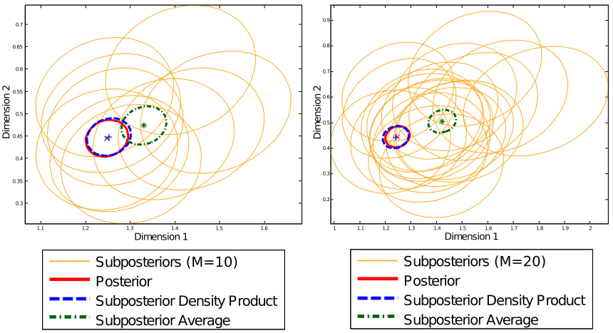
Solution 2: Run MCMC on Subsets of Data
Another solution to parallel MCMC is to simply divide the data into multiple partitions, and then run the full MCMC process on that subset of data. The key idea is to also “distribute” the priors accordingly, and then later combine the subposteriors cleverly.
More formally, the idea is to break down the full posterior into multiple subposteriors :
The original paper introduces four methods to recover the true posterior based on samples from the subposteriors. In this section we describe one, and refer interested readers to the original paper for the rest and for the full derivations.
Here we discuss the method of “asymptotically exact posterior sampling with nonparametric density product estimation”. That is, given samples from a subposterior , write the kernel density estimator as:
Empirically, this results in a consistent full posterior sampling, as compared to the biased naive averaged posterior:
Solution 3: Use Collapsed Gibbs Sampling (CGS)
A third solution makes use of an MCMC algorithm called collapsed Gibbs sampling (CGS).
In CGS framework, we use the following view of the objective, due to
We can parallelize the process in multiple ways, either in data-parallel method, or in model-parallel method.
CGS Data-parallel: Approximate Distributed LDA
In this data-parallel method, we simply split the observations into multiple partitions, have each worker processes each own partition, and then aggregate the update later. This process is illustrated below:

The algorithm is summarized below:
- Split documents into partitions, with their corresponding topic mixture .
- Copy the topic description to each worker
- Each worker runs inference locally and update their parameters
- All workers send back the update to the master server, which aggregates the update
- Master server sends back the updated parameters to all workers, repeating the process.
The problem with this approach is two-fold:
- The overall model is no longer guaranteed to converge, since ergodicity (fully-connectedness) is broken
- Bigger problem: communication time to send parameter updates between master server and the workers could be longer than the computation time.
CGS Model-parallel 1: GraphLab
To solve the communication problem, instead of copying the full model to all workers, we can instead have each worker access only (non-overlapping) portions of the model model parallel method. The question is then: how do we split the model?
Based on the GraphLab framework, we can represent the observations as a bipartite graph between documents and words. And then using vertex cut algorithm we can find partitions of the full graph, which can then be send to different workers to do inference locally in parallel. This is illustrated in the following figure:

This helps eliminate the need to do global synchronization of , since each worker now process disjoint sets of words (and documents). However, the vertex cut problem for graph partitioning is an NP-complete, and existing algorithms take significant amount of time to get good partitions. In this light, LightLDA was proposed.
CGS Model-parallel 2: LightLDA
The idea of LightLDA is still to do model-parallel instead of data-parallel method, but using a much simpler partitioning compared to GraphLab framework. The idea is to split the matrix block-wise, and then rotate the blocks in each iterations, as illustrated below:
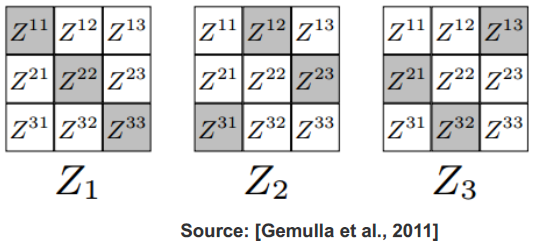
The caveat of this approach is on load imbalance: some documents could have a higher frequency of certain words, causing a worker to be overloaded compared to other workers. In a practical system, these things need to be addressed, for example, by grouping documents by word frequency.
In summary, model-parallel approach is quite desirable over data-parallel for this task because it reduces dependency between workers, since the workers will not step on each other’s toes while making updates locally, since the parameter space assigned to them are disjoint, unlike in data-parallel case.
Challenges of Distributed Systems for ML
Here we discuss some considerations when designing real-world distributed systems. To start, there are two big challenges:
- Networks are slow, compared with local data processing.
- Identical machines rarely perform equally: Hotter machines, vibrating machines, network used by others, other users using computations, etc. All these factors may affect the efficeincy of the machines.
Pay attention to system aspects: bandwidth, latenty, partitioning and scheduling. These variables are not constants but probabilities, and thus there is no such thing as ideal systems behavior.
How difficult is data/model-parallelism? Data parallelism is challenging but manageable. On the contrary, model parallelism is not because naive way usually does not work. That’s why we need schedule.
Intrinsic properties of ML programs
ML programs have some distinct characteristics: First, unlike traditional programs we have some error tolerance. Seoncd, it has dynamic structural dependency. Third, the convergence might be non-uniform. Thus, the design of parallelism of distributed systems for ML programs must take all of them into consideration.
There are mainly two challenges in data parallelism: partial synchronicity and straggler tolerance. Existing ways to cope with them are either safe but slow (BSP), or fast but risky (Async). Stale sync seems to be the middle-ground between bulk and async and thus might worth more exploring.
Theory of Real Distributed ML systems
A little bit Theory of real distributed ML systems is also important. There are three types of convergence guarantees:
- Regret/Expectation bounds on parameters, which is convergence progress per iteration
- Probabilistic bounds on parameters, which is similar to the regret bound but usually stronger
- Variance bounds on parameters, which measures the stability near optimum or convergence
E(SSP) Regret Bound is commonly used. Important to note the interrelation between and . Why does E(SSP) converge? The intuition is that E(SSP) approximates the sequiential ordering of the work. Despite the re-ordering, over the long run E(SSP) is equivalent to sequential execution. That is a good exmaple of how influence of each factor would differ in differnt systems, which cope with delays in differnt ways.
In conclusion, Real-world distributed systems are never ideal. There are in general two solutions: Bounded-Asynchronous Parallel (BAP) and Scheduled Model Parallelism (SMP). Both have advantages and disadvantages, which the theoretical analysis can help us understand better.