Lecture 22: Bayesian non-parametrics

Motivation

Clustering

Bayesian non-parametrics used to be a popular topic in machine learning. The topic is not as popular right now but it is still useful since it’s connected to a wide range of techniques we use today; for example, Gaussian Process can be applied to DNNs to make the layers infinitely wide.

Let’s start from a simpler problem (clustering). We already know a number of algorithms to solve this problem. Cluster analysis or clustering is the task of grouping a set of objects in such a way that objects in the same group (called a cluster) are more similar (in some sense) to each other than to those in other groups (clusters). Algorithms we’ve seen before (e.g. K-means, GMMs) solves if the number of groups was specified.

However, in the real world, identifying the optimal number of clusters is still an open problem. In a two dimensional case, we can usually identify the number of clusters through direct visualization, but it becomes hard to tell when the data is high-dimensional. Nevertheless, we can choose k (number of groups) through some heuristics by comparing the results of different k values, or compactness measures such as intra-cluster distances and inter-cluster distances, but these methods make the problem even harder by inducing an objective/measure that is different from the original object the algorithm tries to optimize.

Moreover, when we are dealing with streaming data (e.g. new/media analysis), the clusters change every day. The algorithm constantly needs to delete and add clusters. People often run K-means on the data every day to accommodate changes, but this induces “the mapping problem”, since outputs of different K-means instances may not be aligned (i.e. Cluster 1 today might correspond to cluster 2 tomorrow).

From GMM to Bayesian Mixture Model

We first start from the formulation of a Mixture of Gaussian (over infinite data) for the clustering problem:

This above GMM is known as a parametric model. We estimate fixed number of parameters from the data.

A Bayesian way of estimating the mixing weights and mixture parameters is to put a prior on them and integrate them out and then do MLE.

For convenience we use conjugate priors. Note that \pi follows a multinomial distribution, so the conjugate prior is a Dirichlet prior. For \mu,\Sigma which parametrize a Gaussian, there is also a conjugate prior known as the Normal-inverse-Wishart distribution.

Note that we still have no clue how to estimate K, and therefore K is normally treated as a hyperparameter determined during tuning.

The Dirichlet distribution

Reason for examining the Dirichlet distribution

The Dirichlet distribution is a distribution over vectors with values between 0 and 1 that sum to 1, meaning these vectors can be used as the probabilities of a discrete distribution. Because of this, the Dirichlet distribution can be seen as a distribution over distributions.

Details of the Dirichlet distribution

The Dirichlet distribution is defined as

where:

• [\alpha_0 … \alpha_k] are the parameters of the Dirichlet distribution. \alpha_k \geq 0, and \sum_k \alpha_k \gt 0.
• [\pi_0 … \pi_k] are the values the Dirichlet distribution describes the probability of. \sum_k \pi_k = 1, and can be seen as members of the K-1 standard simplex (generalized triangle).

Properties of the Dirichlet distribution

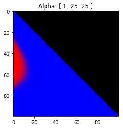
• Probability is evenly distributed when \alpha_k = 1 for all k.
• \alpha_k values less than 1 spread the probability away from the center.
• \alpha_k values greater than 1 gather the probability in the center.
• If the value of \alpha_i is greater than \alpha_j, probability will gather more towards vertex j of the simplex.

Expectation:

The Dirichlet distribution is the conjugate prior to the multinomial and categorical distributions.

Dirichlet distribution as a distribution over distributions

Vectors sampled from the Dirichlet distribution can be used to represent distributions over the parameters of other distributions. For example, each probability in a sampled vector could be associated with the mean and variance of a normal distribution, and that normal distribution could itself be used to produce the parameters of another distribution. In this way, the Dirichlet distribution can act as a distribution over distributions of parameters.

Operations on the Dirichlet distribution

The dimension of the Dirichlet distribution can be modified while maintaining some properties of the distributions it describes.

Collapsing

If (\pi_1,…,\pi_k) \sim Dirichlet(\alpha_1,…,\alpha_k), then

(\pi_1 + \pi_2, \pi_3,…,\pi_k) \sim Dirichlet(\alpha_1 + \alpha_2, \alpha_3,…,\alpha_k)

Splitting

If (\pi_1,…,\pi_k) \sim Dirichlet(\alpha_1,…,\alpha_k) and

(\theta_1,…,\theta_m) \sim Dirichlet(\alpha_1 \beta_1,…,\alpha_1 \beta_m), then

(\pi_1 \theta_1,…,\pi_1 \theta_m, \pi_2,…,\pi_k) \sim Dirichlet(\alpha_1 \beta_1,…,\alpha_1 \beta_m, \alpha_2,…,\alpha_k)

Renormalization

If (\pi_1,…,\pi_k) \sim Dirichlet(\alpha_1,…,\alpha_k) then

\frac {(\pi_2,…,\pi_k)} {\sum^K_{k=2} \pi_k} \sim Dirichlet(\alpha_2,…,\alpha_k)

Parametric vs non-parametric

In this class, we started with parametric models, which assume all data can be represented with a fixed, finite number of parameters. Models of this type include Gaussian Mixture Models (GMM), generalized linear models (GLMs) with exponential families and so on.

On the other hand, number of parameters of non-parametric models can grow with sample size and may be random. An example of pure non-parameteric method is kernel density estimation, where the estimation of the probability density function(pdf) of a random variable is made solely based on a finite sample of data points and some parameters including bandwidth determining the smoothness and a kernel function for weighting the distance from the observations to a particular value the random variable may take. However, non-parametric models are sometimes cumbersome to estimate and are inflexible, especially for data with strong patterns such as those with clusters.

Bayesian non-parametrics is an approach combining the advantages of both parametric and non-parametric modeling. This type of model also allows infinite number of parameters in that the prior is a device defining a random distribution on an infinite space of possible parameters. But the finite dataset that the model will fit will only use a finite subset of those parameters. Given the Bayesian setting, we can integrate out the intermediate layers of random variables if using conjugate-priors, leaving just the hyper-parameters and the data. In this way, we bypass the need to specify the infinite space and can still do inference. By using this type of methods, we can marginalize on something hard to operationalize, focus on only on the more intuitive and direct example hyperparameters and still achieve the same statistical effect of infinite modeling.

The Dirichlet process

Background

By using Bayesian non-parametrics for mixture models, we can write down the posterior probability of the observation as the following: p(x_n \mid\pi,{\mu_k},{\Sigma_k})=\sum_{k=1}^{\infty}\pi_k \ \mathcal{N}(x_n \mid \mu_k,\Sigma_k). Instead of using a finite number of possible clusters, here we use \infty. But we should bear in mind that actually a finite subset of them will be used. Dirichlet prior allows us implicitly define an infinte number of parameters and not necessarily store or maintain them.

Construct an appropriate prior

The process of construction starts with a 2-dimensional Dirichlet distribution paramterized by \alpha. We then split each dimenstion to get K dimensions. For example, a 4-dimensional Dirichlet can be obtained by sampling a pair of beta parameters and apply them to the 2 components according to the splitting rule. By repeating the process, we can finally have a K-dimensional Dirichlet distribution parametrized by \alpha, the concentration parameter, and K. As K goes to infinity, we get a vector with infinitely many components. This operation allows us to extrapolate a finite Dirchlet into infinite without increasing the number of parameters.

The Dirichlet process

Considering a mixture model, given a Dirichlet prior \pi with potentially infinte number of dimensions, we accompany the infinite number of weights with infinite number of centroids drew from a distribution H on some space \Omega, e.g. a Gaussian distribution on the real line. Each sample from H will be discrete and corresponding to 1 dimension in the prior \pi. Then G:=\sum_{k=1}^{\infty}\pi_k\delta_{\theta_k} is a discrete infinite distribution over \Omega, with \delta_{\theta_k} as an indicator for a particular element equivalent to \theta_k. Intuitively, when H is Gaussian, the distribution looks like a set of spikes whose positions determined by Gaussian H and the hights determined by the weights \pi.

The discrete distribution enables sampling centroids with some clustering effect. This cannot be achieved with sampling from a continuous distribution such as Gaussian, since every sample will differ from each other. While with sampling from the Dirichlet process, chances are same posititions will be repeatively sampled.

Sample from the Dirichlet process

We call the point masses in the resulting distribution ‘atoms’ and the corresponding weights ‘sizes’. ‘Sizes’ are determined by the concentration parameter \alpha. Sampling from bigger \alpha leads to atoms spread out more.

Properties of the Dirichlet process

Sampling from Dirichlet process results in partitions of \Omega, which is the space of H. The partition is discrete and difffernt mass is assigned for different partite. Denote the base measure for partite A_1 as H(A_1). Then the mass assigned for each partitie follows the Dirichlet distribution \textbf{Dir}(\alpha H(A_1),..,\alpha H(A_k)), where \alpha is the concentration parameter, i.e.(P(A_1),…,P(A_k))\sim\textbf{Dir}(\alpha H(A_1),..,\alpha H(A_k)). k can \infty.

Through this, we don’t need to express the infinity of the dimentionality in the partition. Instead, we can express by a finite number of partitions, say k-1 and put all the rest into the last single partition.

Conjugacy of the Dirichlet process

Using the conjugacy property of \textbf{Dir}(\alpha H(A_1),..,\alpha H(A_k)), we can express the posterior distribution of the partitions after seeing an example easily. For example, if we see an observation in the J^{th}, then the posterior distribution of (P(A_1),…,P(A_j),…,P(A_k)) follows \textbf{Dir}(\alpha H(A_1),…,\alpha H(A_j) + 1,…,\alpha H(A_k)). Intuitively, we can understand it as a prenormalized mass \alpha H(A_j) plus an evidence. In general, this is written as G \mid X_1 = x \sim DP(\alpha + 1, \frac{\alpha H + \delta_x}{\alpha +1}).

Predictive distribution

Using Dirichlet Process (DP), we can define a easy and handy predictive distribution. Instead of maintaining (P(A_1),…,P(A_j),…,P(A_k)) which is high dimensional, we can use Bayesian trick to integrate out variables and make sampling easier. Suppose we start from nothing. Operationally, we want to do point-sampling of an atom in the space \Omega.

Unlike k-means where we predefined the number of clusters k and then put all data in, here we process each data point one by one. For the first data point, we start by a new cluster and sample a parameter \theta_1 for that cluster. Then we have our first partition: \theta_1 and everything else \theta^c. Let \pi_1 be the size of atom at \theta_1. Then the combined mass of all the other atoms is \pi_* =1-\pi_1. For the distribution over these masses, the prior is (\pi_1, \pi_* ) \sim \textbf{Dir}(0,\alpha). Given H is continuous, the mass of a particular point is 0. After assigning the first data point to the first cluster, the posterior becomes (\pi_1, \pi_* ) \mid X_1=\theta_1 \sim \textbf{Dir}(1,\alpha).

The second data point can have 2 choices, either join the existing cluster or a new cluster. We have

Thus, P(X_2=\theta_k \mid X_1=\theta_1)=\frac{1}{1+\alpha} if k=1 or \frac{\alpha}{1+\alpha} for new k. Note that here we use the posterior after seeing the first data point as prior for the second data point. And the posterior after seeing the second will be used as the prior for the third data point. Say for the second data point, we choose to start a new cluster and sample a new parameter \theta_2 for that cluster. Let \pi_2 be the size of the atom \theta_2. For the third data point, we use the posterior from seeing the second point (\pi_1,\pi_2,\pi_* ) \mid X_1 = \theta_1, X_2=\theta_2 \sim \textbf{Dir}(1,1,\alpha) as the prior. Using the same integration trick, we integrate out \pi = (\pi,\pi_2,\pi_* ) and have P(X_3 = \theta_k \mid X_1=\theta_1, X_2=\theta_2)=\mathbb{E}_{\textbf{Dir}(1,1,\alpha)} [\pi_k]. That is to say, P(X_3 = \theta_k \mid X_1=\theta_1, X_2=\theta_2) equals to \frac{1}{2+\alpha} if k=1 or k=2 and equals to \frac{\alpha}{2+\alpha} for new k.

By applying the integration trick over \pi, we can focus on the prior distribution from the last step, which is parametrized by the number of clusters seeing so far and the counts for data points belonging to each cluster and \alpha. In general, if m_k is the number of times we have seen X_i=k and K is the total number of observed values. We have:

Thus, P(X_{n+1}=\theta_k \mid X_1,..,X_n) equals \frac{m_k}{n+\alpha}, the weight defines by the k-th atom, if k \leq K and it equals to \frac{\alpha}{n+\alpha}, an residual probability, for yet another new cluster. In this way, we can keep attributing labels of new data points purely depending on observed data points and the concentration parameter \alpha. \pi are not needed and we don’t need to worry about sampling \pi. However, we still need to try a few numbers to pick \alpha.

Metaphors for the Dirichlet process

There are many ways to visualize the Dirichlet process. Three common metaphors are the Pólya urn scheme, the Chinese restaurant process, and the stick-breaking process.

Pólya urn scheme

In the Pólya urn scheme (also called the Blackwell-MacQueen urn scheme), imagine we have an urn initially containing a black ball of mass \alpha. To generate each sample X_n, sample a ball from the urn with probability proportional to its mass. The color of the ball is the partition that X_n comes from. If the ball is black, choose a new previously-unseen color for the sample, and return the black ball and a unit-mass ball of that new color to the urn. If the ball is not black, just return it and another unit-mass ball of the same color to the urn.

Then, after sampling n balls, the joint distribution of the balls’ colors (i.e. the cluster the balls belong to) follows a Dirichlet process.

From this scheme, we can also easily see the self-reinforcing property that the Dirichlet process exhibits: new samples are more likely to be drawn from partitions that already have many existing samples.

The Chinese restaurant process

The Chinese restaurant process is an equivalent description of the Pólya urn scheme.

Imagine a restaurant with an infinite number of tables, all initially empty. The first customer enters the restaurant, and picks a table to sit at. When the (n-1)-th customer enters, they either 1) sit at an occupied table k with probability \frac{m_k}{n + \alpha}, where m_k is the number of people that are currently sitting at table k, or 2) start a new table with probability \frac{\alpha}{n + \alpha}. We can see that this description is equivalent to the Pólya urn scheme above.

Note on Exchangeability

Even though the two descriptions above have a notion of an order of the drawn samples, it turns out that the distribution over the partitions of the first N samples does not depend on the order of the samples. However this does not mean the samples are independent, since we have seen the self-reinforcing property of the Dirichlet process - samples tend to be drawn from partitions that already have many existing samples.

Distributions that do not depend on the order of the samples are called exchangeable distributions.

De Finetti’s theorem states that if a sequence of observations are exchangeable, then there must exist a distribution given which the samples are i.i.d. In this case, the samples are i.i.d. given the Dirichlet process.

The stick-breaking process

The two metaphors above primarily show the distribution of the data points among the resulting partitions. The stick-breaking process shows how the partitions of the DP can be constructed, along with their associated parameters, to give the parameters of the resulting distribution G.

Imagine we begin with a stick of unit length, which represents our total probability. We then repeatedly break off fractions of the stick, and assign parameters to each broken-off fraction according to our base measure.

Concretely, to construct the k-th partition:

1. Sample a Beta(1, \alpha) random variable \beta_k \in [0, 1].
2. Break off a fraction \beta_k of the remaining stick. This gives us the k-th partition. We can calculate its atom size \pi_k using the previous fractions \beta_1, …, \beta_k.
3. Sample a random parameter \theta_k for the partition for this atom from our base measure G_0.
4. Recur on the remaining stick.

In summary,

The stick-breaking metaphor shows us how we can approximate a Dirichlet process. The final distribution G is obtained from a weighted sum of the sampled parameters \theta_k, weighted by the atom size \pi_k. Since the atom sizes of the created partitions in the stick-breaking process are monotonically decreasing, we can get a good approximation of G by just using the first k sampled parameters and atom sizes.