Collision
Resolution
Introduction
In this lesson we will discuss several collision resolution strategies. The key thing in hashing is to find an easy to compute hash function. However, collisions cannot be avoided. Here we discuss three strategies of dealing with collisions, linear probing, quadratic probing and separate chaining.
Linear Probing
Suppose that a key hashes into a position that is already occupied. The simplest strategy is to look for the next available position to place the item. Suppose we have a set of hash codes consisting of {89, 18, 49, 58, 9} and we need to place them into a table of size 10. The following table demonstrates this process.
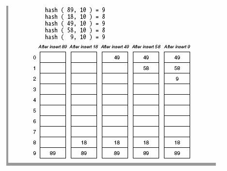
Table Courtesy of Weiss Data Structures
Book
The first collision occurs when 49 hashes to the same location with index 9. Since 89 occupies the A[9], we need to place 49 to the next available position. Considering the array as circular, the next available position is 0. That is (9+1) mod 10. So we place 49 in A[0]. Several more collisions occur in this simple example and in each case we keep looking to find the next available location in the array to place the element. Now if we need to find the element, say for example, 49, we first compute the hash code (9), and look in A[9]. Since we do not find it there, we look in A[(9+1) % 10] = A[0], we find it there and we are done. So what if we are looking for 79? First we compute hashcode of 79 = 9. We probe in A[9], A[(9+1)%10]=A[0], A[(9+2)%10]=A[1], A[(9+3)%10]=A[2], A[(9+4)%10]=A[3] etc. Since A[3] = null, we do know that 79 could not exists in the set.
Lazy Deletion
When collisions are resolved using linear probing, we need to be careful about removing elements from the table as it may leave holes in the table. One strategy is to do what’s called “lazy deletion”. That is, not to delete the element, but place a marker in the place to indicate that an element that was there is now removed. In other words, we leave the “dead body” there, even though it is not part of the data set anymore. So when we are looking for things, we jump over the “dead bodies” until we find the element or we run into a null cell. One drawback in this approach is that, if there are many removals (many “dead bodies”), we leave a lot of places marked as “unavailable” in the array. So this could lead to a lot of wasted spaces. Also we may have to frequently resize the table to find more space. However, considering space is cheap, “lazy deletion” is still a good strategy. The following figure shows the lazy deletion process.

Clustering in Linear
Probing
One problem in linear probing is that clustering could develop if many of the objects have hashed into places that are closer to each other. If the linear probing process takes long due to clustering, any advantage gained by O(1) lookups and updates can be erased. One strategy is to resize the table, when the load factor of the table exceeds 0.7. The load factor of the table is defined as number of occupied places in the table divided by the table size. The following image shows a good key distribution with little clustering and clustering developed when linear probing is used for a table of load factor 0.7.
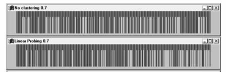
Table Courtesy of Weiss Data Structures
Book
Quadratic Probing
Although linear probing is a simple process where it is easy to compute the next available location, linear probing also leads to some clustering when keys are computed to closer values. Therefore we define a new process of Quadratic probing that provides a better distribution of keys when collisions occur. In quadratic probing, if the hash value is K , then the next location is computed using the sequence K + 1, K + 4, K + 9 etc..
The following table shows the collision resolution using quadratic probing.
Separate Chaining
The last strategy we discuss is the idea of separate chaining. The idea here is to resolve a collision by creating a linked list of elements as shown below.

In the picture above the objects, “As”, “foo”, and “bar” all hash to the same location in the table, that is A[0]. So we create a list of all the elements that hash into that location. Similarly, all other lists indicate keys that were hashed into the same location. Obviously a good hash function is needed so that keys can be evenly distributed. Because any uneven distribution of keys will neutralize any advantage gained by the concept of hashing. Also we must note that separate chaining requires dynamic memory management (using pointers) that may not be available in some programming languages. Also manipulating a list using pointers is generally more complicated than using a simple array.