idx to idx = (1:1:N)' and see what happens. 
Exercise 3: Cycle between the three test cases, cs = 1, 2, 3.


Example 2: Try running 'vincent.m'.  You will be given a choice of patterns, and the code
will extrapolate these patterns automatically.  This script reconstructs some of the results in
Fast Kernel Learning for Multidimensional Pattern Extrapolation.

Do not worry if there are occasional warnings that LCG has not converged.  The
optimization will proceed normally.  The warnings can be resolved by adjusting
the tolerance and maximum number of iterations.  We have set these values for a
good balance of accuracy and efficiency, not minding if LCG occasionally does
not converge to within the specified precision.

Some example output:





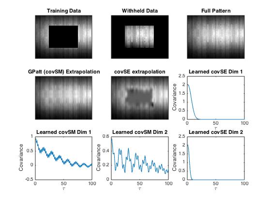
Note the learned spectral mixture kernels.  It would be difficult to know to a priori hard code
kernels like these.  The learned structure is interpretable and enables good predictions and
extrapolation. 

Exercise 1:  Extrapolations are produced with spectral mixture kernels and SE kernels. 
Try adding a Matern kernel to this demo.  It will do better on the letters example than
an SE kernel, but not as well as the spectral mixture kernel on larger missing regions.

Exercise 2:  Study the initialisation script spectral_init.m.   This is a basic and
robust initialisation for spectral mixture kernels.  Can you think of other initialisations
which might offer even better performance?

Exercise 3:  Reproduce Figure 1j in Wilson et. al, NIPS 2014, showing the initial
and learned weights against the initial and learned frequencies.
 
Exercise 4: Adjust this script to your own patterns and general purpose regression
problems, such as the land surface temperature forecasting in Wilson et. al, NIPS 2014.

Author: Seth Flaxman 4 March 2015

clear all, close all
% This comes from a dataset giving the locations of trees by type in a forest in
% Michigan [D. J. Gerrard 1969]. I obtained it from the R package spatstat
% as follows (run this code in R:

% library(spatstat)
% hicks <- split(lansing)$hickory
% write.table(data.frame(hicks),"hickories.csv", row.names=F,col.names=F,sep=",")

xy = csvread('hickories.csv');
plot(xy(:,1),xy(:,2),'.')

% create the "computational grid"
n1 = 32; n2 = 32;
x1 = linspace(0,1.0001,n1+1); x2 = linspace(-0.0001,1,n2+1);
xg = {(x1(1:n1)+x1(2:n1+1))'/2, (x2(1:n2)+x2(2:n2+1))'/2};

i = ceil((xy(:,1)-x1(1))/(x1(2)-x1(1)));
j = ceil((xy(:,2)-x2(1))/(x2(2)-x2(1)));
counts = full(sparse(i,j,1));

% setup the GP
cv = {@covProd,{{@covMask,{1,@covSEiso}},{@covMask,{2,@covSEisoU}}}};
cvGrid = {@covGrid, { @covSEiso,  @covSEisoU}, xg};
hyp0.cov = log([.1  1 .1]);
y = counts(:);

X = covGrid('expand', cvGrid{3});
Idx = (1:length(y))';
lik = {@likPoisson, 'exp'};
hyp0.mean = .5;

tic
hyp1 = minimize(hyp0, @gp, -100, @infLaplace, @meanConst, cv, lik, X, y);
toc
exp(hyp1.cov)

Function evaluation      0;  Value 1.114380e+03
Function evaluation      5;  Value 1.104834e+03
Function evaluation      8;  Value 1.098415e+03
Function evaluation     12;  Value 1.097589e+03
Function evaluation     16;  Value 1.097445e+03
Function evaluation     18;  Value 1.097417e+03
Function evaluation     23;  Value 1.096718e+03
Function evaluation     26;  Value 1.096703e+03
Function evaluation     30;  Value 1.096424e+03
Function evaluation     33;  Value 1.096419e+03
Function evaluation     35;  Value 1.096419e+03
Function evaluation     37;  Value 1.096419e+03
Function evaluation     46;  Value 1.096419e+03
Elapsed time is 300.589011 seconds.

ans =

    0.0815    0.6522    0.0878

tic
hyp2 = minimize(hyp0, @gp, -100, @infGrid_Laplace, @meanConst, cvGrid, lik, Idx, y);
toc
exp(hyp2.cov)

Function evaluation      0;  Value 1.151583e+03
Function evaluation     12;  Value 1.124633e+03
Function evaluation     14;  Value 1.116309e+03
Function evaluation     17;  Value 1.115676e+03
Function evaluation     20;  Value 1.115373e+03
Function evaluation     23;  Value 1.115308e+03
Elapsed time is 41.778548 seconds.

ans =

    0.2346    0.5824    0.1100

The models learned slightly different hyperparameters. Are the likelihoods different?

fprintf('Log-likelihood learned w/out Kronecker: %.04f\n', gp(hyp1, @infLaplace, @meanConst, cv, lik, X, y));
fprintf('Log-likelihood learned with Kronecker: %.04f\n', gp(hyp2, @infLaplace, @meanConst, cv, lik, X, y));

% and what about the likelihood we actually calculated in infGrid_Laplace,
% using the Fiedler bound?
fprintf('Log-likelihood with Kronecker + Fiedler bound: %.04f\n', gp(hyp2, @infGrid_Laplace, @meanConst, cvGrid, lik, Idx, y));

% let's compare our posterior predictions--to save time, we'll use infGrid_Laplace to
% make predictions in both cases (this won't hurt the accuracy, as we explain in the paper.)
[Ef1 Varf1 fmu1 fs1 ll1] = gp(hyp1, @infGrid_Laplace, @meanConst, cvGrid, lik, Idx, y, Idx, y);
[Ef2 Varf2 fmu2 fs2 ll2] = gp(hyp2, @infGrid_Laplace, @meanConst, cvGrid, lik, Idx, y, Idx, y);

figure(1); imagesc([0 1], [0 1], (reshape(Ef1,32,32)')); set(gca,'YDir','normal'); colorbar;
figure(2); imagesc([0 1], [0 1], (reshape(Ef2,32,32)')); set(gca,'YDir','normal'); colorbar;

Log-likelihood learned w/out Kronecker: 1096.4188
Log-likelihood learned with Kronecker: 1100.3819
Log-likelihood with Kronecker + Fiedler bound: 1115.3084

now let's exploit the grid structure to get a finer resolution map we'll also switch covariances, just for fun.

hyp.cov = log([.3  1 .2 1]);
lik = {@likPoisson, 'exp'}; hyp.lik = [];
mean = {@meanConst}; hyp.mean = .5;

n1 = 64; n2 = 64;
x1 = linspace(0,1.0001,n1+1); x2 = linspace(-0.0001,1,n2+1);
xg = {(x1(1:n1)+x1(2:n1+1))'/2, (x2(1:n2)+x2(2:n2+1))'/2};

% binning y = histcn(xy,x1,x2);
i = ceil((xy(:,1)-x1(1))/(x1(2)-x1(1)));
j = ceil((xy(:,2)-x2(1))/(x2(2)-x2(1)));
counts = full(sparse(i,j,1));
y = counts(:);
xi = (1:numel(y))';
cov = {@covGrid, { {@covMaterniso,5},  {@covMaterniso,5}}, xg};

opt.cg_maxit = 400; opt.cg_tol = 1e-2;
inf_method = @(varargin) infGrid_Laplace(varargin{:},opt);

tic
  hyp2 = minimize(hyp, @gp, -100, inf_method, mean, cov, lik, xi, y(:));
toc
exp(hyp2.cov)

% let's compare our posterior predictions
% since we don't care about variance, we can save memory by doing this:
[post nlZ dnlZ] = infGrid_Laplace(hyp2, mean, cov, lik, xi, y(:));
post.L = @(x) 0*x;
ymu = gp(hyp2, @infGrid_Laplace, mean, cov, lik, xi, post, xi);
figure(3), imagesc([0 1], [0 1], reshape(ymu,size(counts))'),
hold on;
set(gca,'YDir','normal');
plot(xy(:,1),xy(:,2),'w.');
colorbar
hold off

Function evaluation      0;  Value 1.954834e+03
Function evaluation      6;  Value 1.946841e+03
Function evaluation      8;  Value 1.940877e+03
Function evaluation     11;  Value 1.940012e+03
Function evaluation     14;  Value 1.938218e+03
Function evaluation     17;  Value 1.936884e+03
Function evaluation     20;  Value 1.934900e+03
Function evaluation     22;  Value 1.933195e+03
Elapsed time is 187.843026 seconds.

ans =

    0.3051    0.7512    0.1636    0.7512