Constraint Satisfaction Problems
Learning Objectives
Describe definition of CSP problems and its connection with general search problems
Formulate a real-world problem as a CSP
Describe and implement backtracking algorithm
Define arc consistency
Describe and implement forward checking and AC-3
Explain the differences between MRV and LCV heuristics
Understand the complexity of general binary CSP and tree-structured binary CSP
Discuss how ethical problems can be approached using CSP concepts/formulation
Search and CSPs
Search serves two main purposes:
planning: sequence of actions
the path to the goal is most important
paths and costs have various depths
heuristics give problem-specific guidance
identification: assignments to variables
the goal is the most important (not the path)
all paths are are at the same depths (for some formulations)
Previously, when we learned about search algorithms, we were primarily concerned with finding a path from our start state to our goal state.
Now, we will look into constraint satisfaction problems (CSPs), which are primarily identification problems.
Standard Search Problems have
State: arbitrary data structure
Goal Test: any function over states
Successor Function: anything
Specifications for CSPs
State: variables \(X_i\) with values from domain \(D_i\)
Goal Test: set of constraints specifying allowable combinations of values for subsets of variables
CSP Formulation
Whenever we formulate a CSP, we need to identify the following: set of variables \(X\), set of domains \(D\), and set of constraints \(C\).
Variable \(X_i\): Factored representation of each state.
Domain \(D_i\): Set of allowable values for variable \(X_i\).
Constraint \(C_i\): Consists of tuple of variables that participate in the constraint, and relation that defines the values that those variables can take on.
There are a variety of types of constraints:
Unary Constraints: Involve a single variable. It is equivalent to reducing domains. For map coloring it would be \(A \neq Green\)
Binary Constraints: Involve pairs of variables. For map coloring, an example would be \(A \neq B\)
Higher Order Constraints: Involve three or more variables
Example
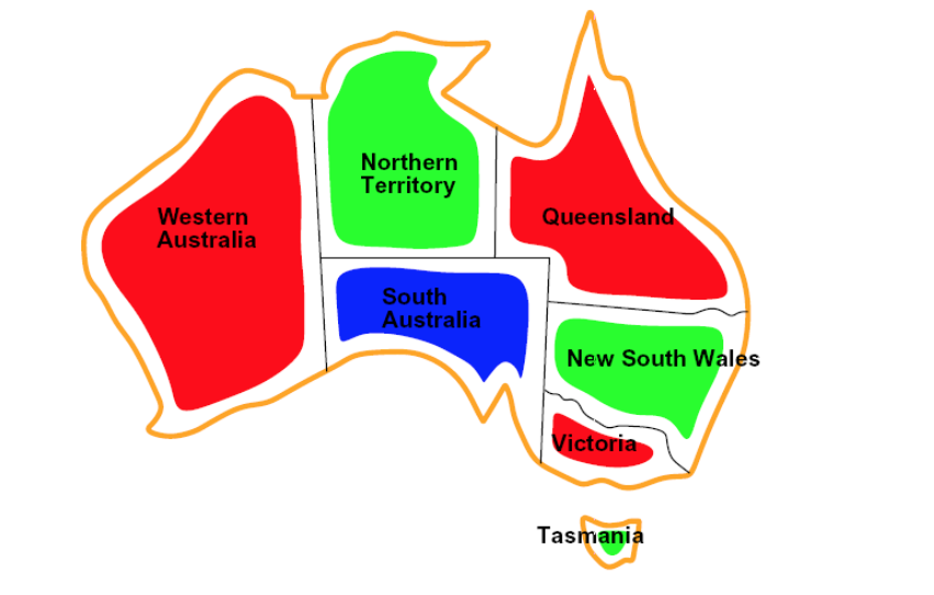
Variables: WA, NT, Q, NSW, V, SA, T
Domain: \(\{\)red, green, blue\(\}\)
Constraints: adjacent regions must have different colors
Explicit Constraint Example: (WA, NT) \(\in \{\)(red, green), (red, blue), (blue, green), (blue, red), (green, red), (green, blue)\(\}\)
Implicit Constraint Example: WA \(\neq\) NT
Solution: assignments satisfying all constraints
Example: \(\{\) WA=red, NT=green, Q=red, NSW=greeen, V=red, SA=blue, T=green\(\}\)
Constraint Graph
In a binary CSP problem, each constraint relates (at most) two variables. We can represent this problem as a binary constraint graph, where
Each node corresponds to a variable
An edge between any two nodes indicates a constraint between them
General purpose CSP algorithms take advantage of the graph's structure to speed up search.
Consider our CSP problem formulation for the map coloring example from earlier. The corresponding constraint graph is below:

Note that node T (corresponding to Tasmania) has no edges connecting it to other nodes in the CSP graph. This indicates that coloring Tasmania is an independent subproblem.
Algorithms for Solving CSPs
Naive Algorithm
Our first attempt at formulating a CSP into a search problem might be as follows:
States are partial assignments of the variables. Full assignments are goal states.
Actions involve adding an assignment var = value, where var is an unassigned variable, to a partial assignment. An action is legal if it does not result in a assignment that violates constraints.
We could then run any one of our standard search algorithms to find a satisfying assignment.
Let's conduct a cost analysis. Let \(n\) be the number of variables, and \(d\) be the size of the domain. At depth 0, there is a branching factor of \(nd\), as we choose among \(n\) variables to assign, then choose 1 of \(d\) values. At depth 1 there is a branching factor of \((n - 1)d\), as there is one less variable to assign. At depth i we then have a branching factor of \((n - i)d\). To choose among the leaves of the search tree, we have the following multi-step process:
assignment = {}
for i in 0, ..., n-1:
    assignment <- one of the children of the current assignment
    ((n - i)d options)
Then the number of leaves is \(\prod_{i=0}^{n-1}\big((n - i)d\big) = d^n\prod_{i=0}^{n-1}(n - i) = n!d^n\). But wait - the number of solutions to this CSP should be bounded by \(d^n\), the number of ways to assign \(n\) variables with each having \(d\) options. Many of these goal states are equivalent because the order of assignment of variables doesn't matter - actions in this domain are commutative. With this observation we can restrict the search to choosing between \(d\) options to assign to a single variable at each level, giving us the expected number of leaves \(d^n\).
Backtracking Search
The following algorithm formalizes running depth-first search with the more restrictive formulation we arrived at in the last section. We repeatedly choose an unassigned variable and cycle through possible assignments of that variable. If no consistent assignments can be found of the remaining variables for any assignment of the considered variable, we indicate failure, backtracking to the previous assignment.
def backtracking-search(csp):
    csp: a CSP
    Output: solution (variable assignment) or failure
    return backtracking({}, csp)

def backtrack(assignment, csp):
    if assignment complete:
        return assignment
    var = select_unassigned_variable(csp)
    for value in order_domain_values(var, csp):
        if value consistent with assignment:
            assignment[var] = value
            result = backtrack(assignment, filter(csp))
            if result != FAILURE:
                return result
        remove assignment[var]
    return FAILURE
Since backtracking is an uninformed algorithm for solving CSPs, it can be slow. We can solve CSPs faster by considering the following:
Filtering: By filtering out inconsistent values from domains, can we detect inevitable failure early?
Ordering: Which variables should be assigned next (
select_unassigned_variable)? In what order should its values be tried (order_domain_values)?Structure: Can we exploit the problem structure?
Filtering Algorithms
The main idea behind filtering algorithms for CSPs are to
keep track of domains for unassigned variables
eliminate bad domain values (i.e., values that violate constraints) along the way
Most filtering algorithms try to achieve arc consistency.
Note that filtering algorithms are added within the backtracking search algorithm above.
Let \(A\) and \(B\) be unassigned variables in our CSP with a binary constraint between them.

An arc \(A \rightarrow B\) is consistent if and only if for all values \(a\) remaining in \(A\)'s domain, there's some corresponding value \(b\) remaining in \(B\)'s domain such that \(a\) and \(b\) satisfy all constraints between \(A\) and \(B\).
We refer to \(A\) as the tail, and \(B\) as the head.
If arc consistency is not satisfied at some point in our process of solving the CSP, we enforce it by removing values from the current domain of \(A\) until the arc is consistent.
# Enforces consistency of A -> B, i.e., removes inconsistent values from A's domain if necessary
def enforce_arc_consistency(A, B):
    A, B: variables of the CSP
    Output: boolean denoting whether we updated domain of A
    removed = False
    for each a in domain[A]:
        if no value b in domain[B] allows (a, b) to satisfy the constrain between A and B:
            delete a from domain[A]
            removed = True
return removed Complexity: Enforcing arc consistency for a single arc \(A \rightarrow B\) is \(O(d^2)\).
Recall from the pseudocode that in the context of backtracking search, we would run a filtering algorithm on our current CSP after assigning a value to a variable.
We'll now delve into two specific filtering algorithms.
Forward Checking
Forward checking enforces consistency of the arcs corresponding to a single variable, i.e., the arcs between that variable and its immediate neighbors.
def forward_check(csp, x):
    csp: a CSP with variables X1, X2, ..., Xn
    x: one of the variables in csp
    Output: the same CSP, but with potentially reduced domains
    for Xi in neighbors[x]:
        enforce_arc_consistency(Xi, x)
    return csp
Note: Since this forward checking pseudocode take as input a single variable, in the context of the backtracking search algorithm, we would likely call
These are minor implementation details that aren't super important.
The main shortcoming of forward checking is it does not provide early detection for all failures which may be induced by a domain change/assignment.
Complexity: A single run of forward checking (i.e., for a single variable/a single call to the above function) is \(O(nd^2)\).
AC-3
Forward checking only checks arcs pointing to newly assigned variables. AC-3 checks even more.
AC-3 enforces consistency of arcs corresponding to a particular variable, and then enforces arc consistency for any variables whose domains were affected in the process. This effectively propagates any domain changes outward from the original variable (for which consistency was enforced) to its neighbors, neighbors' neighbors, etc.
def AC-3(csp):
    csp: a CSP with variables X1, X2, ..., Xn
    Output: the same CSP, but with potentially reduced domains
    queue = [(Xi, Xj) for all combinations of i, j in csp (i.e., all arcs in csp)]
    while queue not empty:
        (Xi, Xj) = queue.remove()
        removed = enforce_arc_consistency(Xi, Xj)
        if removed:
            for Xk in neighbors[Xi]:
                queue.add((Xk, Xi))
    return csp
Note that we could alternatively also pass in a single variable \(X\) to AC-3 (like in the provided forward checking implementation), and initialize the queue with just the incoming arcs to \(X\) instead of all arcs in the CSP.
Complexity: A single run of AC-3 is \(O(n^2d^3)\).
We start with all \(O(n^2)\) arcs on the queue.
The number of arcs added to the queue while running AC-3 is bounded by \(O(n^2d)\). This is because at most we can remove \(O(nd)\) values from domains (\(n\) total variables, each with domain of size \(d\)), and would add \(O(n)\) arcs after each removal.
Enforcing arc consistency of each arc is \(O(d^2)\).
Total: \(O(n^2d^3)\)
Ordering
When it comes to picking which variables to assign and which values to assign to them, we have two main heuristics for prioritizing the options. Recall that variables refer to the factored representation of each state, and values refer to the set of allowable values for each variable.
Minimum Remaining Values: pick the variable with the smallest number of remaining assignable values.
Motivation: fail-fast approach. We need to assign all variables a value at some point, so we might as well do the harder variables first. This heuristic allows us to prune the search tree faster and detect whether we need to backtrack earlier.
Least Constraining Value: pick the value that constrains the smallest number of the chosen variable's neighbors.
Motivation: we want just one solution. We don't need to try all combinations of values, just ones that are more likely to be part of a valid solution.