Bayes Nets

Learning Objectives

1. Answer any query from a joint distribution.

2. Construct joint distribution from conditional probability tables using chain rule.

3. Construct joint distribution from Bayes net and conditional probability tables.

4. Construct Bayes net given conditional independence assumptions.

5. Identify conditional independence assumptions from real-world problems.

6. Analyze the computational and space complexity inference on joint distribution.

7. Identify independence relationships in a given Bayes net.

8. Describe why Bayes nets are used in practice.

9. Decide which sampling method is the most appropriate for an arbitrary query.

Bayes Nets: Representation

Answer Query from Conditional Probability Table (CPT)

Given: \(P(E \mid Q), P(Q)\)

Query: \(P(Q \mid e)\)

1. Construct joint distribution (using product rule or chain rule) \[\begin{align*} P(E, Q) &= P(E \mid Q) P(Q) \end{align*}\]

2. Answer query from joint distribution (using conditional probability or marginalization) \[\begin{align*} P(Q \mid e) &= \frac{P(e, Q)}{P(e)} \text{ by conditional probability} \\ &= \frac{P(e, Q)}{\sum_{q} P(e, q)} \end{align*}\]

There are two main problems with using full joint distribution tables as our probabilistic models

• Unless there are only a few variables, the joint is WAY too big to represent explicitly

• Hard to learn (estimate) anything empirically about more than a few variables at a time

This is the motivation behind Bayes nets: a technique for describing complex joint distributions (models) using simple, local distributions (conditional probabilities)

• More properly called graphical models

• We describe how variables locally interact

• Local interactions chain together to give global, indirect interactions

Graphical Model Notation

Nodes: variables (with domains)

• Can be assigned (observed) or unassigned (unobserved)

Arcs: interactions

• Similar to CSP constraints

• Indicate “direct influence” between variables (Note: arrows do not necessarily mean direct causation)

• More formally, they encode conditional dependence between unobserved variables

When constructing the joint probability table for the Bayes Net, we use the following convention: \[P(Node_1,...Node_n) = \prod_{i=1}^n P(Node_i | Parents(Node_i))\] So instead of storing the entire joint probability table, we can store each conditional probability table and save space. Bayes Nets allow us to represent these conditional independence relationships in a concise way.

Example

For the following Bayes nets, write the joint \(P(A, B, C, D, E)\)



The joint probability for this Bayes Net would be as follows: \[P(A, B, C, D, E) = P(A)P(B)P(C|A,B)P(D|B)P(E|C,D)\] This is exponentially smaller than the joint probability if we had none of the independence assumptions given to us in the Bayes Net.

Independence

Conditional Independence and Bayes Ball

Are \(X\) and \(Y\) conditionally independent given evidence variables \(Z\)?

• Yes, if \(X\) and \(Y\) “d-separated” by \(Z\)

• Consider all (undirected) paths from \(X\) to \(Y\)

• No active paths = independence!

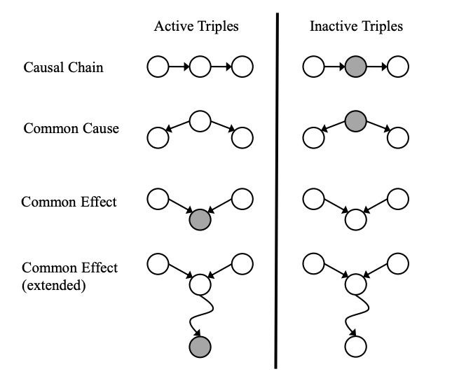
A path is active if each triple along the path is active:

• Causal chain \(X \rightarrow Z \rightarrow Y\) where \(Z\) is unobserved (either direction)

• Common cause \(X \leftarrow Z \rightarrow Y\) where \(Z\) is unobserved

• Common effect (aka v-structure) \(X \rightarrow Z \leftarrow Y\) where \(Z\) or one of its descendents is observed

If all paths between \(X\) and \(Y\) are inactive, \(X \perp\!\!\!\perp Y \mid Z_1, ..., Z_n\).

To answer "Are \(X\) and \(Y\) conditionally independent given evidence variables \(Z\)?", follow the steps below:

1. Shade in \(Z\)

2. Drop a ball at \(X\)

3. The ball can pass through any active path and is blocked by any inactive path (ball can move either direction on an edge)

4. If the ball reaches \(Y\), then \(X\) and \(Y\) are NOT conditionally independent given \(Z\)

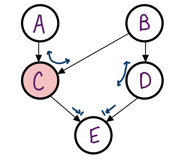
Example

In the Bayes Net from before, is A independent of B given C?

No, the Bayes ball can travel through C.

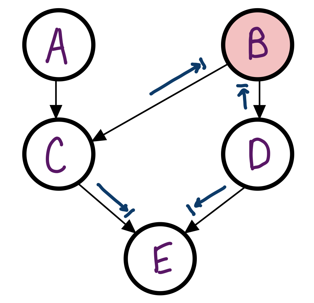
Example

In the Bayes Net from before, is C independent of D given B?

Yes, the Bayes Ball cannot travel through either path to D.

Inference

As seen before in logic, inference is a generic term that refers to answering questions (queries) about variables we’re interested in based on things we know.

Examples of such queries:

• what’s the probability distribution of event \(Q\) based on some observed evidence \(e\)? i.e., \(P(Q \mid e)\)

• what’s the most likely outcome for event \(Q\) based on evidence \(e\)? i.e., \(\text{argmax}_q P(q \mid e)\)

We can answer any generic query about the variables of a Bayes’ net using the following steps:

1. Re-express the query solely in terms of the joint probability (of all variables in the Bayes’ net). This will likely require applying the chain rule and marginalizing (summing over) variables we’re not interested in.

2. Compute the joint probability using the conditional probability tables of the BN (recall that joint = the product of all tables of the BN).

Example

Answer the query \(P(+w \mid +s, -g)\). \[P(+w \mid +s, -g)\] \[= \frac{P(+w, +s, -g)}{P(+s, -g)} \textit{ (chain rule)}\] \[= \frac{\sum_{h} P(h, +w, +s, -g)}{\sum_{h, w} P(h, w, +s, -g)} \textit{ (marginalization)}\] \[= \frac{\sum_{h} P(h)P( +w \mid h)P(+s \mid +w)P( -g \mid +w)}{\sum_{h, w} P(h) P(w \mid h) P(+s \mid w) P(-g \mid w)} \textit{ (joint = product of CPTs)}\] \[= \frac{0.1 * 0.667 * 0.4 * 0.75 + 0.9 * 0.25 * 0.4 * 0.75}{0.1 * 0.667 * 0.4 * 0.75 + 0.9 * 0.25 * 0.4 * 0.75 + 0.1 * 0.333 * 0.2 * 0.5 + 0.9 * 0.75 * 0.2 * 0.5}\] \[=0.553\]

This process is sometimes referred to as enumeration, as we’re essentially enumerating all relevant rows from the full joint distribution to help us answer the query.

Since marginalization is expensive, if the query is a probability distribution, we might elect to hold off calculating the denominator until the very end.

Example

Suppose the above example asked for \(P(W \mid +s, -g)\). After applying the chain rule, I can rewrite this expression as \(\frac{P(W, +s, -g)}{Z}\) or \(\alpha \times P(W, +s, -g)\). Ignoring \(\alpha / Z\) for now, I have the table for \(P(W, +s, -g)\) : \[\begin{array}{|c|c|} \hline P(+w, +s, -g) & 0.0875 \\ \hline P(-w, +s, -g) & 0.0708 \\ \hline \end{array}\] To get the final distribution we want (\(P(W \mid +s, -g)\)), we just need to turn this table into a valid probability distribution which sums to 1 by dividing each entry by the sum of all entries: \[\begin{array}{|c|c|} \hline P(+w \mid +s, -g) & 0.0875 / 0.158 = 0.553 \\ \hline P(-w \mid +s, -g) & 0.0708 / 0.158 = 0.448 \\ \hline \end{array}\] (And we know this is mathematically correct because \(\sum_w P(W, +s, -g) = P(+s, -g)\), which is exactly the denominator we need.)

This concept applies to more complex queries, too, and will come up again in variable elimination below.

We’ll also sometimes specify in the problem that you can use a normalization constant, which means you can just leave your answer in terms of \(\alpha\) or \(Z\) without calculating its actual value. Don’t assume you can do this unless we explicitly say so!

Variable Elimination

Enumeration is expensive, especially as the number of variables in the BN increases. To maximize inference efficiency, we use a method called variable elimination, which aims to reduce the number of computations needed by rearranging terms and summations.

Algorithm:

def variable_elimination(query, e, bn):  
    q = re-express query in terms of bn.CPTs  
    factors = all probability tables in q  
    for v in order(bn.variables):  
        new_factor = make_factor(v, factors)  
        factors.add(new_factor)  
    return normalize(product of all factors)  
      
def make_factor(v, factors):  
    relevant_factors = [remove all f from factors if f depends on v]  
    new_factor = product of all relevant_factors  
    return sum_out(relevant_factors, v)  

*I’ve written this algorithm somewhat differently from the way it’s presented in lecture - feel free to use whichever is more helpful to you.

Example

This example will show the mechanics of performing variable elimination, but not the mathematical calculations. Feel free to fill those in yourself for practice!



Find \(P(H \mid +s)\).

\[P(H \mid +s) = \frac{P(H, +s)}{P(+s)} = \frac{\sum_{w, g}P(H, w, +s, g)}{\sum_{h, w, g}P(h, w, +s, g)} = (\alpha)\sum_{w, g} P(H)P(w \mid H)P(+s \mid w)P(g \mid w)\] (In the last step, we square away the denominator as \(\alpha\) as seen before. We’ll compute it at the end.)



Initial factors: [\(P(H), P(W \mid H), P(+s \mid W), P(G \mid W)\)]

Let’s fix the elimination order \(G, W\).

Eliminating \(G\):

Factors which involve \(G\): \(P(G \mid W)\).

To make a new factor, we first multiply these together: \(P(G \mid W)\) (in lecture Stephanie annotated this as a separate factor itself, i.e., \(f_1(W) = P(g \mid W)\), but we’ll omit this here)

then sum out (eliminate) \(G\): \(f_1(W) = \sum_g P(g \mid W)\). \[\begin{array}{|c|c|} \hline W & f_1(W) \\ \hline +w & \\ \hline -w & \\ \hline \end{array}\]

Current factors: [\(P(H), P(W \mid H), P(+s \mid W), f_1(W)\)]

Eliminating \(W\):

Factors which involve \(W\): \(P(W \mid H), P(+s \mid W), f_1(W)\).

Make a new factor by multiplying these together: \(P(W \mid H) P(+s \mid W) f_1(W)\)

and summing out \(W\): \(f_2(H) = \sum_w P(w \mid H) P(+s \mid w) f_1(w)\). \[\begin{array}{|c|c|} \hline H & f_2(H) \\ \hline +h & \\ \hline -h & \\ \hline \end{array}\]

Current factors: [\(P(H), f_2(H)\)]

To answer the query, normalize \(P(H) f_2(H)\), i.e., factor back in that \(\alpha\) we put to the side before.

\[\begin{array}{|c|c||c|} \hline H & P(H)f_2(H) & P(H \mid +s) \\ \hline +h & a & a / (a + b) \\ \hline -h & b & b / (a + b) \\ \hline \end{array}\] The rightmost column gives us the final answer to our query.

Since we keep intermediate factors (i.e., probability tables) in memory, both the time and space efficiency of variable elimination is largely dependent upon the ordering of variables. Intuitively, we want to eliminate as many variables as possible before computing large sums; therefore, it’s more computationally efficient to eliminate variables with fewer connections first. For instance, in the example above had we eliminated \(W\) first, the resulting factors would have been \(f_1(H, G)\) and \(f_2(H)\). Since the first factor is a function of 2 variables rather than 1, this would require more space and time to compute.

Sampling

With the right variable ordering, variable elimination can help reduce the computational and space complexity of exact inference problems by a lot. However, in the worst case, exact inference is still \(O(2^n)\), where \(n\) is the number of variables.

Therefore, we introduce an approximate inference method known as sampling, which should help us get answers that are "good enough". In each of the following methods, we assume that we have access to the individual probability tables of the Bayes’ Net, and we use some source of randomness (e.g., a random number generator) which simulates picking values for variables.

Prior Sampling

Prior sampling is the most straightforward/baseline kind of sampling. For each variable in the BN, we use a random generator to pick a value for it (e.g., generate a float between 0 and 1 and see where it lies with respect to the distribution defined by that variable’s probability table). We repeat this a number of times we deem sufficient, and then use the numbers of samples seen to calculate the query.

# generates one sample with prior sampling.  
def prior_sample():  
    for i = 1,2,...k:  
        Sample x_i from P(X_i | Parents(X_i))  
    return (x_1, x_2,...x_k)  

As a result, for a BN with variables \(X_1, X_2, \dots, X_n\), the probability of sample \(x_1, x_2, \dots, x_n\) is \[\prod_{i=1}^n P(x_i \mid Parents(X_i)) = P(x_1, x_2, \dots, x_n).\] In other words, the probability distribution we’re estimating here is the joint distribution of all variables (from which we can compute any query).

Example

Each sample is generated with true joint probability of the prior distribution. For instance, one event (+h, +w, +s, +g) is generated with probability of \(0.1*0.667*0.4*0.25 = 0.00667\). This means with large N, we expect 0.667 percent of the samples to be (+h, +w, +s, +g).

Suppose we want to estimate \(P(+h)\), and we generated following 10 samples: \[\begin{array}{|c|c|} \hline \text{sample} & \text{count} \\ \hline (-h, +w, +s, +g) & 4 \\\hline (-h, +w, -s, +g) & 3 \\\hline (+h, +w, +s, +g) & 1 \\\hline (+h, +w, -s, +g) & 2 \\\hline \end{array}\] We estimate probability by \(P(+h) = \sum_w \sum_s \sum_g P(+h, w, s, g)\), and each probability is estimated by counting the event and dividing it by number of samples. For instance, \(P(+h, +w, +s, +g) = 1/10\). Adding up each of the appropriate probability values, we get \(P(+h) = 0.3\), since there are 3 samples with \(+h\) out of 10. Notice it is different from true distribution, 0.1, but our estimated probability from samples will become exact in a large sample limit.

Rejection Sampling

Rejection sampling is exactly the same as prior sampling, only we reject all samples which are inconsistent with the observed evidence in our query so that we only get samples that we want.

def rejection_sample(evidence instantiation):  
  for i = 1,2 ... n:  
      Sample x_i from P(X_i | Parents(X_i))  
      if x_i not consistent with evidence:  
          # Reject: no sample generated in this cycle
          return None   
  return (x_1, x_2,...x_k)

With rejection sampling, the probability of getting a sample that does not agree with our evidence is 0 since we throw away any such samples.

Likelihood-Weighted Sampling

Similar to rejection sampling, in likelihood-weighted sampling we don’t want to end up with samples that are inconsistent with observed evidence. Instead of throwing out samples, however, which is wasteful and even inefficient if the evidence is rare, we fix evidence variables and only sample the other variables. Each sample also comes with a weight \(w\), which is the product of probabilities of each evidence variable taking on its observed value given the values of their parents.

def likelihood_weighted_sample(evidence instantiation):  
  w = 1.0  
  for i = 1,2,...n:  
      if(X_i is an evidence variable):  
          X_i = observation x_i for X_i  
          w = w * P(x_i | Parents(X_i))  
      else:  
          Sample x_i from P(X_i | Parents(X_i))  
  return ((x_1, x_2,...x_n), w)  

The weight of a sample effectively represents the likelihood of the evidence for that sample, and we ultimately multiply it by the sample’s count to make our approximate inferences.

Important: 2 identical samples (i.e., same variable values) will also have the same weights.

Example

Estimate \(P(+h \mid +w, +g)\).

When generating samples, we fix \(W = +w, G = +g\) and sample values for \(H, S\) using some kind of random generator.

Suppose we generated the following 10 samples: \[\begin{array}{|c|c|} \hline \text{sample} & \text{count} \\ \hline (-h, +w, +s, +g) & 1 \\\hline (-h, +w, -s, +g) & 2 \\\hline (+h, +w, +s, +g) & 4 \\\hline (+h, +w, -s, +g) & 3 \\\hline \end{array}\]

By nature of the sample-generating algorithm, each sample comes with a weight \(w = \prod_{e_i} P(e_i \mid parents(e_i))\), where \(e_i\) are the evidence instantiations provided. Intuitively, our sample counts help estimate \(\prod_{v_i} P(v_i \mid parents(v_i))\), where \(v_i\) are our sampled values for the non-evidence variables. Then, to estimate the joint distribution, we simply multiply these weights by the ratio of sample counts to the total number of samples drawn for all variables \(x_i\) - i.e., the joint.

\[\begin{array}{|c|c|c|c|c|} \hline \text{sample} & \text{ratio} & \text{weight} & \text{estimated } P(sample) \\ \hline (-h, +w, +s, +g) & 1/10 & P(+w \mid -h)P(+g \mid +w) & \frac{1}{10}P(+w \mid -h)P(+g \mid +w) = a\\ \hline (-h, +w, -s, +g) & 1/5 & P(+w \mid -h)P(+g \mid +w) & \frac{1}{5}P(+w \mid -h)P(+g \mid +w) = b\\ \hline (+h, +w, +s, +g) & 2/5 & P(+w \mid +h)P(+g \mid +w) & \frac{2}{5}P(+w \mid +h)P(+g \mid +w) = c\\ \hline (+h, +w, -s, +g) & 3/10 & P(+w \mid +h)P(+g \mid +w) & \frac{3}{10}P(+w \mid +h)P(+g \mid +w) = d\\ \hline \end{array}\] We now have an estimated version of the joint distribution, but only with variable value settings consistent with the evidence. \[P(+h \mid +w, +g) = \frac{P(+h, +w, +g)}{P(+w, +g)} = \frac{\sum_s P(+h, +w, s, +g)}{P(+w, +g)} \approx \frac{c + d}{a + b + c +d}\] where in the final step we approximate \(P(+w, +g)\) as the sum of entries in the above table since all entries have \(+w, +g\).

Gibbs Sampling

The last time of sampling that we talk about is Gibbs sampling. In Gibbs sampling, it allows us to take turns sampling the variable that we want to learn about. This allows us to consider both "upstream" and "downstream" variables. In likelihood weighted sampling, it only conditions on upstream variables that are being conditioned on so the weights obtained can often times be very small. Since then the sum of the weights would be small, the number of "effective" samples would be low as well. Gibbs works to fix this issue.

def gibbs_sample(full instantiation x_1...x_n):  
  1. Start with an arbitrary instantiation consistent with the evidence  
  2. Sample 1 variable at a time, conditioned on all others  
  3. Keep repeating for a long time  

By repeating the two steps many times, we are guaranteed that the resulting sample will come from the correct distribution. The basic idea is that Gibbs allows us to get an approximate sample based on the distribution in an efficient manner. For a full proof of why this works and/or for an example, we recommend you rewatch the part of Lecture when Stephanie goes through it.

You can find an interactive web demo for Gibbs sampling here.