Comparing LCFR and ZLIFO


Next: The Value of Separable-Threat
Up: Experimental Comparison of Flaw
Previous: The Value of Least-Cost
Comparing LCFR and ZLIFO
We next turn to a direct comparison of LCFR and ZLIFO. Gerevini
and Schubert compared these strategies on only a few problems. To get
a more complete picture of the performance of both LCFR and ZLIFO, we
ran them both on all the problems from our three problem sets.
The data for the basic problem set is shown in Figure  .
We have sorted the problems by the difference between the node counts
produced by LCFR and ZLIFO. Thus, problems near the left-hand side
of the graph are those for which LCFR generated a smaller search
space, while problems near the right-hand side are the ones on which
ZLIFO had a space advantage. We omit problems which neither strategy
could solve.
As can be seen, on some problems (notably R-Test2, Move-Boxes, and
Monkey-Test2), LCFR generates a much smaller search space than ZLIFO,
while on other problems (notably Get-Paid4, Hanoi, Uget-Paid4, and
Uget-Paid3), ZLIFO generates a much smaller search space. These are
problems on which LCFR also did worse than the
strategies mentioned above in Section  .
.
As we noted earlier, one of the major changes between UCPOP v.2 and
v.4 is that v.4 puts the elements of a new set of open conditions onto
the flaw list in the reverse order from that of v.2.
This ordering may make a difference, particularly for LIFO-based
strategies. Indeed, other researchers have suggested that one reason
a LIFO-based strategy may perform well is because it can exploit the
decisions made by the system designers in writing the domain
operators, since it is in some sense natural to list the most
constraining preconditions of an operator first [Williamson & Hanks, 1996].
We therefore also collected data for a modified version of UCPOP, in
which the preconditions for each step are entered onto the open
condition in the reverse of the order in which they would normally be
entered. We discuss the results of this modification in more detail
in the next two sections, but for now, we simply present the node
counts for LCFR and ZLIFO with the reversed precondition insertion, in
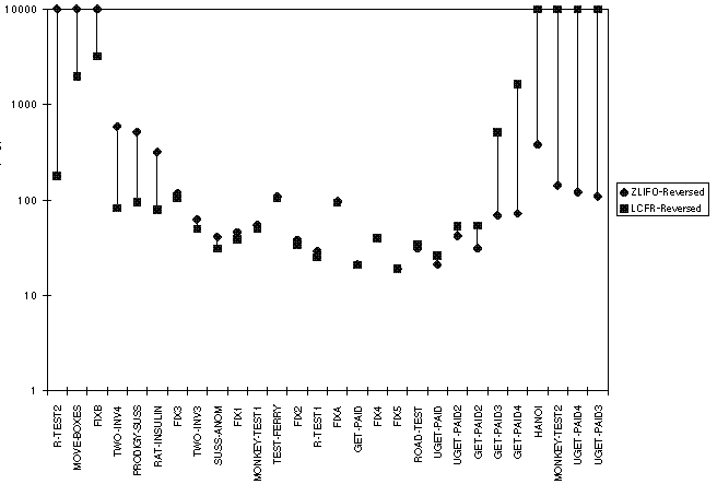
Figure  . As can be seen, there are a few problems on
which reversing the precondition ordering has a significant effect
(notably FIXB and MonkeyTest2), but by and large LCFR and ZLIFO showed
the same relative performance.
 Figure: Basic Problems: Node Counts for LCFR and ZLIFO
 Figure: Basic Problems: Node Counts for LCFR and ZLIFO with
Reversed Precondition Insertion
For the problems in the basic set, it is difficult to discern an
obvious pattern of performance. In contrast to what Gerevini and
Schubert suggest, there does not seem to be a clear correlation
between the difficulty of the problem, measured in terms of nodes
generated, and the relative performance of LCFR and ZLIFO. (In
fact, it is a little difficult to determine which strategy's
node-count should serve as the measure of difficulty.) On the other
hand, it is true that in the aggregate, ZLIFO generates smaller search
spaces than LCFR on the basic problems. With the default precondition
ordering, ZLIFO obtains an average %-overrun of 212.62, while LCFR
obtains 647.57. With reverse ordering, ZLIFO's average %-overrun is
244.24, while LCFR's is 914.87. The fact that LCFR's relative
performance is worse when the preconditions are entered in the reverse
direction results primarily from its failure on MonkeyTest2 in the
reverse direction.
The Trains data is scant.
Neither LCFR nor ZLIFO can solve the hardest problem,
Trains3, regardless of whether the preconditions are entered in the
default or the reverse order. (In fact, none of the strategies we studied were able to
solve Trains3.)
But, at least when the preconditions are entered in the default order, ZLIFO can solve
Trains2, and LCFR cannot. With reverse precondition insertion, neither
strategy can solve Trains2.
The data are shown in Figure  . Note that LCFR's
performance is essentially the same for both node-selection strategies shown.
Finally, the Tileworld data, for the default order of precondition
insertion, is shown in Figure  . Here is the only place
in which LCFR clearly generates smaller search spaces than ZLIFO. We
have not also plotted the data for reverse precondition insertion,
because most of the strategies are not affected by this change. There
is however, one very notable exception: with reversed insertion, ZLIFO
(with S+OC+.1UC+F) does much better--indeed, it does as well as
LCFR. We return to the influence of precondition ordering on the
Tileworld problems in
Section
  .
.
For now, however, it is enough to observe that our experiments show
that ZLIFO does tend to generate smaller search spaces than LCFR.
It does so on the basic problem set, regardless of the order of
precondition insertion, it does so on Trains for one ordering (and
does no worse than LCFR on the other ordering), and it does as well as
LCFR for the Tileworld problems when the preconditions are inserted in
the reverse order. The only exception is the Tileworld problem set
when the preconditions are inserted in default order: there LCFR does
better.
 Figure: Trains Problems: Node Counts for LCFR and ZLIFO
 Figure: Tileworld Problems: Node Counts for LCFR and ZLIFO


Next: The Value of Separable-Threat
Up: Experimental Comparison of Flaw
Previous: The Value of Least-Cost
TOM Conversion
Wed Jun 25 17:40:58 EDT 1997
 .
We have sorted the problems by the difference between the node counts
produced by LCFR and ZLIFO. Thus, problems near the left-hand side
of the graph are those for which LCFR generated a smaller search
space, while problems near the right-hand side are the ones on which
ZLIFO had a space advantage. We omit problems which neither strategy
could solve.


