2.4 Histories and Runs

An agent reasoning about summary information to make planning decisions at abstract levels needs to first be able to reason about CHiPs. In this section we complete the semantics of CHiPs by describing how they affect the state over time. Because an agent can execute a plan in many different ways and in different contexts, we need to be able to quantify over possible worlds (or histories) where agents fulfill their plans in different ways. After defining a history, we define a run as the transformation of state over time as a result of the history of executions. The formalization of histories and runs follows closely to that of RAK in describing multiagent execution.

A state of a world, $s$, is a truth assignment to a set of propositions, each representing an aspect of the environment. We will refer to the state as the set of true propositional variables. A history, $h$, is a tuple $\langle E, s_I\rangle$. $E$ is the set of all plan executions of all agents occurring in $h$, and $s_I$ is the initial state of $h$ before any plan begins executing. So, a history $h$ is a hypothetical world that begins with $s_I$ as the initial state and where only executions in $E(h)$ occur. In particular, a history for the manufacturing domain might have an initial state as shown in Figure 1 where all parts and machines are available, and both transports are free. The set of executions $E$ would contain the execution of $produce\_H$, $maintenance$, $move\_parts$, and their subexecutions.

A run, $r$, is a function mapping a history and time point to states. It gives a complete description of how the state of the world evolves over time, where time ranges over the positive real numbers.

Axiom 1   $$r(h,0) = s_I$$

Axiom 2   $$\begin{array}{@{}l@{}l@{}l} v \in r(h,t>0) \Leftrightarrow &... ...(\neg v \in post(p') \wedge t_f(e_{p'}) = t)) \par \end{array}$$

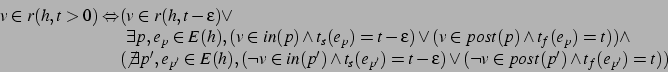
Axiom 1 states that the world is in the initial state at time zero. Axiom 2 states that a predicate $v$ is true at time $t$ if it was already true beforehand, or a plan asserts $v$ with an incondition or postcondition at $t$, but (in either case) no plan asserts $\neg v$ at $t$. If a plan starts at $t$, then its inconditions are asserted right after the start, $t+\epsilon$, where $\epsilon$ is a small positive real number. Axiom 2 also indicates that both inconditions and postconditions are effects.

The state of a resource is a level value (integer or real). For consumable resource usage, a task that depletes a resource is modeled to instantaneously deplete the resource (subtract $usage$ from the current state) at the start of the task by the full amount. For non-consumable resource usage, a task also depletes the usage amount at the start of the task, but the usage is restored (added back to the resource state) at the end of execution. A task can replenish a resource by having a negative $usage$. We will refer to the level of a resource $res$ at time $t$ in a history $h$ as $r(res,h,t)$. Axioms 3 and 4 describe these calculations for consumable and non-consumable resources, respectively.

Axiom 3   $$\begin{array}{@{}l@{}l@{}l} r(consumable\_res,h,t) = r(consu... ..._{e_p\in E(h), t_s(e_p)=t} usage(p,consumable\_res) \end{array}$$

Axiom 4   $$\begin{array}{@{}l@{}l@{}l} r(nonconsumable\_res,h,t) = &r(n... ..._p\in E(h), t_f(e_p)=t} usage(p,nonconsumable\_res) \end{array}$$

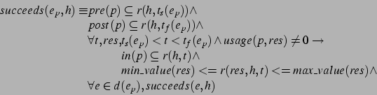
Now that we have described how CHiPs change the state, we can specify the conditions under which an execution succeeds or fails. As stated formally in Definition 1, an execution succeeds if: the plan's preconditions are met at the start; the postconditions are met at the end; the inconditions are met throughout the duration (not including the start or end); all used resources stay within their value limits throughout the duration; and all executions in the decomposition succeed. Otherwise, the execution fails.

Definition 1   $$\begin{array}{@{}l@{}l} succeeds(e_p, h) \equiv &pre(p) \sub... ...nd{array} \\ &\forall e \in d(e_p), succeeds(e,h) \end{array}$$