|
Journal of Artificial Intelligence Research, 28 (2007) 453-515. Submitted 8/06; published 4/07
© 2007 AI Access Foundation and Morgan Kaufmann Publishers. All rights reserved.
Bradley J. Clement
Edmund H. Durfee
Anthony C. Barrett
Jet Propulsion Laboratory, Mail Stop: 126-347
Pasadena, CA 91109 USA
brad.clement@jpl.nasa.gov
Electrical Engineering and Computer Science Department
University of Michigan,Ann Arbor, MI 48109 USA
durfee@umich.edu
Jet Propulsion Laboratory, Mail Stop: 126-347
Pasadena, CA 91109 USA
tony.barrett@jpl.nasa.gov
The judicious use of abstraction can help planning agents to identify key interactions between actions, and resolve them, without getting bogged down in details. However, ignoring the wrong details can lead agents into building plans that do not work, or into costly backtracking and replanning once overlooked interdependencies come to light. We claim that associating systematically-generated summary information with plans' abstract operators can ensure plan correctness, even for asynchronously-executed plans that must be coordinated across multiple agents, while still achieving valuable efficiency gains. In this paper, we formally characterize hierarchical plans whose actions have temporal extent, and describe a principled method for deriving summarized state and metric resource information for such actions. We provide sound and complete algorithms, along with heuristics, to exploit summary information during hierarchical refinement planning and plan coordination. Our analyses and experiments show that, under clearcut and reasonable conditions, using summary information can speed planning as much as doubly exponentially even for plans involving interacting subproblems.
Abstraction is a powerful tool for solving large-scale planning and scheduling problems. By abstracting away less critical details when looking at a large problem, an agent can find an overall solution to the problem more easily. Then, with the skeleton of the overall solution in place, the agent can work additional details into the solution [Sacerdoti 1974, Tsuneto, Hendler, Nau, 1998]. Further, when interdependencies are fully resolved at abstract levels, then one or more agents can flesh out sub-pieces of the abstract solution into their full details independently (even in parallel) in a ``divide-and-conquer'' approach [Korf, 1987, Lansky, 1990, Knoblock, 1991].
Unfortunately, it is not always obvious how best to abstract large, complex problems to achieve these efficiency improvements. An agent solving a complicated, many-step planning problem, for example, might not be able to identify which of the details in earlier parts will be critical for later ones until after it has tried to generate plans or schedules and seen what interdependencies end up arising. Even worse, if multiple agents are trying to plan or schedule their activities in a shared environment, then unless they have a lot of prior knowledge about each other, it can be extremely difficult for one agent to anticipate which aspects of its own planned activities are likely to affect, and be affected by, other agents.
In this paper, we describe a strategy that balances the benefits and risks of abstraction in large-scale single-agent and multi-agent planning problems. Our approach avoids the danger of ignoring important details that can lead to incorrect plans (whose execution will fail due to overlooked interdependencies) or to substantial backtracking when abstract decisions cannot be consistently refined. Meanwhile, our approach still achieves many of the computational benefits of abstraction so long as one or more of a number of reasonable conditions (listed later) holds.
The key idea behind our strategy is to annotate each abstract operator in a plan hierarchy with summary information about all of its potential needs and effects under all of its potential refinements. While this might sound contrary to the purpose of abstraction as reducing the number of details, in fact we show that it strikes a good balance. Specifically, because all of the possibly relevant conditions and effects are modeled, the agent or agents that are reasoning with abstract operators can be absolutely sure that important details cannot be overlooked. However, because the summary information abstracts away details about under which refinement choices conditions and effects will or will not be manifested, and information about the relative timing of when conditions are needed and effects achieved, it still often results in an exponential reduction in information compared to a flat representation.
Based on the concept of summary information, this paper extends the prior work summarized below and in Section 8 to make the following contributions:
This ability to coordinate at abstract levels rather than over detailed plans allows each of the agents to retain some local flexibility to refine its operators as best suits its current or expected circumstances without jeopardizing coordination or triggering new rounds of renegotiation. In this way, summary information supports robust execution systems such as PRS [Georgeff Lansky, 1986], UMPRS [Lee, Huber, Durfee, Kenny, 1994], RAPS [Firby, 1989], JAM [Huber, 1999], etc. that interleave the refinement of abstract plan operators with execution.
Our approach also extends plan coordination (plan merging) techniques [Georgeff, 1983, Lansky, 1990, Ephrati Rosenschein, 1994] by utilizing plan hierarchies and a more expressive temporal model. Prior techniques assume that actions are atomic, meaning that an action either executes before, after, or at exactly the same time as another. In contrast, we use interval point algebra [Vilain Kautz, 1986] to represent the possibility of several actions of one agent executing during the execution of one action of another agent. Because our algorithms can choose from alternative refinements in the HTN dynamically in the midst of plan coordination, they support interleaved local planning, multiagent coordination, and concurrent execution.
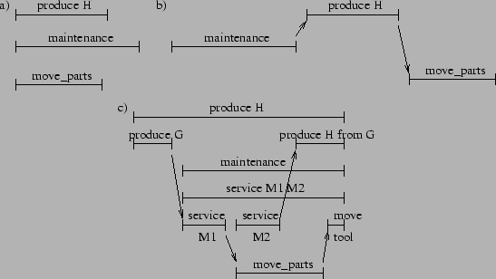
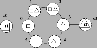
As a running example to motivate this work, consider a manufacturing plant where a production manager, a facilities manager, and an inventory manager each have their own goals with separately constructed hierarchical plans to achieve them. However, they still need to coordinate over the use of equipment, the availability of parts used in the manufacturing of other parts, storage for the parts, and the use of transports for moving parts around. The state of the factory is shown in Figure 1. In this domain, agents can produce parts using machines M1 and M2, service the machines with a tool, and move parts to and from the shipping dock and storage bins on the shop floor using transports. Initially, machines M1 and M2 are free for use, and the transports (transport1 and transport2), the tool, and all of the parts (A through E) shown in their storage locations are available.
The production manager is responsible for creating a part H
using machines M1 and M2. Either M1 and M2 can consume parts A and B
to produce G, and M2 can produce H from G. The production manager's
hierarchical plan for manufacturing H involves using the transports to
move the needed parts from storage to the input trays of the
machines, manufacturing G and H, and transporting H back to storage.
This plan is shown in Figure 2. Arcs through
subplan branches mean that all subplans must be executed.
Branches without arcs denote alternative choices
to achieving the parent's goal. The decomposition of ![]() is similar to that of
is similar to that of ![]() .
.
The facilities manager services each machine by equipping it
with a tool and then calibrating it. The machines are unavailable for
production while being serviced. The facilities manager's
hierarchical plan branches into choices of servicing the machines in
different orders and uses the transports for getting the tool from storage
to the machines (Figure 3). The decomposition of
![]() is similar to that of
is similar to that of ![]() .
.
The parts must be ``available'' on the space-limited shop floor in order for an agent to use them. Whenever an agent moves or uses a part, it becomes unavailable. The inventory manager's goal is just to move part C to the dock and move D and E into bins on the shop floor (shown in Figure 4).
To accelerate the coordination of their plans, each factory manager can analyze his hierarchical plan to derive summary information on how each abstract plan operator can affect the world. This information includes the summary pre-, post-, and in-conditions that intuitively correspond to the externally required preconditions, externally effective postconditions, and the internally required conditions, respectively, of the plan based on its potential refinements. Summary conditions augment state conditions with modal information about whether the conditions must or may hold and when they are in effect. Examples are given at the end of Section 3.2.
Once summary information is computed,
the production and inventory managers each could send this information
for their top-level plan to the facilities manager. The
facilities manager could then reason about the top-level summary
information for each of their plans to determine that if the
facilities manager serviced all of the machines before the production
manager started producing parts, and the production manager finished
before the inventory manager began moving parts on and off the dock,
then all of their plans can be executed (refined) in any
way, or ![]() .
Then the facilities manager could instruct the others to add communication
actions to their plans so that they synchronize their actions appropriately.
.
Then the facilities manager could instruct the others to add communication
actions to their plans so that they synchronize their actions appropriately.
This top-level solution maximizes robustness in that the choices in
the production and facilities managers' plans are preserved, but the
solution is inefficient because there is no concurrent activity--only
one manager is executing its plan at any time. The production manager
might not want to wait for the facilities manager to finish maintenance and could negotiate for a solution
with more concurrency. In that case, the facilities manager could
determine that they could not overlap their plans in any way without risking
conflict (![]() ).
However, the summary information could tell them
that there might be some way to overlap their plans
(
).
However, the summary information could tell them
that there might be some way to overlap their plans
(![]() ),
suggesting that a search for a solution with more concurrency (at the cost of perhaps committing to specific refinement choices) has hope of success.
In this case, the facilities manager could request the production manager for
the summary information of each of
),
suggesting that a search for a solution with more concurrency (at the cost of perhaps committing to specific refinement choices) has hope of success.
In this case, the facilities manager could request the production manager for
the summary information of each of ![]() 's subplans, reason
about the interactions of lower level actions in the same way, and
find a way to synchronize the subplans for a more fine-grained
solution where the plans are executed more concurrently. We give an algorithm for finding such solutions in Section 5.
's subplans, reason
about the interactions of lower level actions in the same way, and
find a way to synchronize the subplans for a more fine-grained
solution where the plans are executed more concurrently. We give an algorithm for finding such solutions in Section 5.
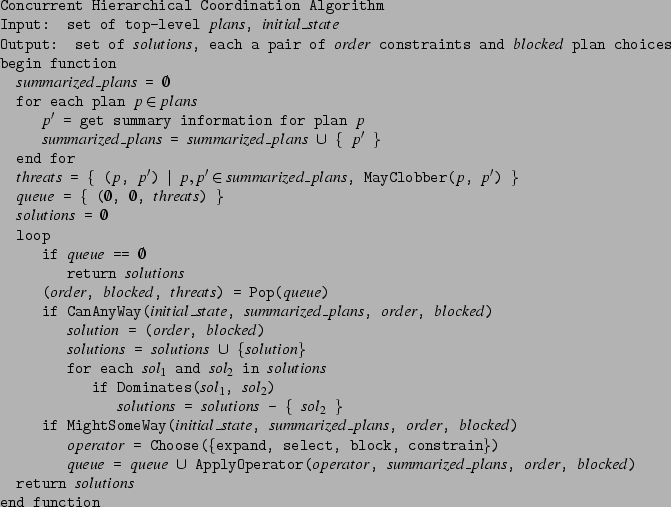
We first formally define a model of a concurrent hierarchical plan, its execution, and its interactions (Section 2). Next, we describe summary information for propositional states and metric resources, mechanisms determining whether particular interactions must or may hold based on this information, and algorithms for deriving the information (Section 3). Built upon these algorithms are others for using summary information to determine whether a set of CHiPs must or might execute successfully under a set of ordering constraints (Section 4). These in turn are used within a sound and complete multilevel planning/coordination algorithm that employs search techniques and heuristics to efficiently navigate and prune the search space during refinement (Section 5). We then show how planning, scheduling, or coordinating at abstract levels can exponentially improve the performance of search and execution (Section 6). We provide experimental results demonstrating that the search techniques also greatly reduce the search for optimal solutions (Section 7). Finally, in Section 8 we differentiate our approach from related work that we did not mention elsewhere and conclude.
A representation of temporal extent in an HTN is important not only for modeling concurrently executing agents but also for performing abstract reasoning with summary information. If an agent is scheduling abstract actions and can only sequentially order them, it will be severely restricted in the kinds of solutions it can find. For example, the agent may prefer solutions with shorter makespans, and should seek plans with subthreads that can be carried out concurrently.
In this section we define concurrent hierarchical plans (CHiPs), how the state changes over time based on their executions, and concepts of success and failure of executions in a possible world, or history. Because we later define summary information and abstract plan interactions in terms of the definitions and semantics given in this section, the treatment here is fairly detailed (though for an even more comprehensive treatment, see [Clement, 2002]). However, we begin by summarizing the main concepts and notation introduced, to give the reader the basic gist.
A CHiP (or plan
![]() ) is mainly differentiated from an HTN by including in its
definition inconditions,
) is mainly differentiated from an HTN by including in its
definition inconditions, ![]() ,
(sometimes called ``during conditions'') that affect (or assert a
condition on) the state just after the start time of
,
(sometimes called ``during conditions'') that affect (or assert a
condition on) the state just after the start time of ![]() (
(![]() ) and
must hold throughout the duration of
) and
must hold throughout the duration of ![]() . Preconditions (
. Preconditions (![]() )
must hold at the start, and postconditions (
)
must hold at the start, and postconditions (![]() ) are asserted at
the finish time of
) are asserted at
the finish time of ![]() (
(![]() ). Metric resource (
). Metric resource (![]() ) consumption
(
) consumption
(![]() ) is instantaneous at the start time and, if the resource
is defined as non-consumable,
is instantaneously restored at the end. The decompositions of
) is instantaneous at the start time and, if the resource
is defined as non-consumable,
is instantaneously restored at the end. The decompositions of ![]() (
(![]() ) is in the
style of
) is in the
style of ![]() /
/![]() tree, having either a partial ordering
(
tree, having either a partial ordering
(![]() ) or a choice of child tasks that each can have their own
conditions.
) or a choice of child tasks that each can have their own
conditions.
An execution ![]() of
of ![]() is an instantiation of its start
time, end time, and decomposition. That is, an execution nails down
exactly what is done and when. In order to reason about plan
interactions, we can quantify over possible histories, where each history
corresponds to a combination of possible executions of the
concurrently-executing CHiPs for a partial ordering over their
activities and in the context of an initial state.
A run (
is an instantiation of its start
time, end time, and decomposition. That is, an execution nails down
exactly what is done and when. In order to reason about plan
interactions, we can quantify over possible histories, where each history
corresponds to a combination of possible executions of the
concurrently-executing CHiPs for a partial ordering over their
activities and in the context of an initial state.
A run (![]() ) specifies the state at
time
) specifies the state at
time ![]() for history
for history ![]() .
.
Achieve, clobber, and undo interactions are
defined in terms of when the executions of some plans assert a positive literal
![]() or negative literal
or negative literal ![]() relative to when
relative to when ![]() is required by another
plan's execution for a history. By looking at the literals achieved, clobbered,
and undone in the set of executions in
a history, we can identify the conditions that must hold prior to the
executions in the history as external preconditions and those that must hold after
all of the executions in the history as external postconditions.
is required by another
plan's execution for a history. By looking at the literals achieved, clobbered,
and undone in the set of executions in
a history, we can identify the conditions that must hold prior to the
executions in the history as external preconditions and those that must hold after
all of the executions in the history as external postconditions.
The value of a metric resource at time ![]() (
(![]() ) is
calculated by subtracting from the prior state value the usage of all
plans that start executing at
) is
calculated by subtracting from the prior state value the usage of all
plans that start executing at ![]() and (if non-consumable) adding back
usages of all that end at
and (if non-consumable) adding back
usages of all that end at ![]() . An execution
. An execution ![]() of
of ![]() fails if a
condition that is required or asserted at time
fails if a
condition that is required or asserted at time ![]() is not in the state
is not in the state ![]() at
at ![]() , or if the value of a resource (
, or if the value of a resource (![]() ) used by the plan
is over or under its limits during the execution.
) used by the plan
is over or under its limits during the execution.
In the remainder of this section, we give more careful, detailed descriptions of the concepts above, to ground these definitions in firm semantics; the more casual reader can skim over these details if desired. It is also important to note that, rather than starting from scratch, our formalization weaves together, and when necessary augments, appropriate aspects of other theories, including Allen's temporal plans allen:83b, Georgeff's theory for multiagent plans georgeff:84, and Fagin et al.'s theory for multiagent reasoning about knowledge RAK.
A concurrent hierarchical plan ![]() is a tuple
is a tuple ![]() ,
, ![]() ,
,
![]() ,
, ![]() ,
, ![]() ,
, ![]() ,
, ![]() .
. ![]() ,
, ![]() , and
, and
![]() are sets of literals (
are sets of literals (![]() or
or ![]() for some propositional
variable
for some propositional
variable ![]() ) representing the preconditions, inconditions, and
postconditions defined for plan
) representing the preconditions, inconditions, and
postconditions defined for plan ![]() .1
.1
We borrow an existing model of metric resources [Chien, Rabideu, Knight, Sherwood, Engelhardt, Mutz,
Estlin, Smith, Fisher, Barrett, Stebbins, Tran, 2000b, Laborie Ghallab, 1995].
A plan's ![]() is a function mapping from resource variables to an amount used. We write
is a function mapping from resource variables to an amount used. We write ![]() to indicate the amount
to indicate the amount ![]() uses of resource
uses of resource ![]() and sometimes treat
and sometimes treat ![]() as a set of pairs
as a set of pairs ![]() .
A metric resource
.
A metric resource ![]() is a tuple
is a tuple ![]() ,
, ![]() ,
, ![]() .
The min and max values can be integer or real
values representing bounds on the capacity or amount available. The
.
The min and max values can be integer or real
values representing bounds on the capacity or amount available. The ![]() of the resource is either consumable or
non-consumable.
For example, fuel
and battery energy are consumable resources because, after use, they
are depleted by some amount. A non-consumable resource is available
after use (e.g. vehicles, computers, power).
of the resource is either consumable or
non-consumable.
For example, fuel
and battery energy are consumable resources because, after use, they
are depleted by some amount. A non-consumable resource is available
after use (e.g. vehicles, computers, power).
Domain modelers typically only specify state conditions and resource usage for primitive actions
in a hierarchy. Thus, the conditions and usage of a CHiP are used to derive summary conditions,
as we describe in Section 3.4, so that algorithms can reason about any action in the hierarchy.
In order to reason about plan hierarchies as
and/or trees of actions, the ![]() of plan
of plan ![]() , or
, or ![]() , is given
a value of either
, is given
a value of either ![]() ,
, ![]() , or
, or ![]() . An
. An ![]() plan is a
non-primitive plan that is accomplished by carrying out all of its
subplans. An
plan is a
non-primitive plan that is accomplished by carrying out all of its
subplans. An ![]() plan is a non-primitive plan that is accomplished
by carrying out exactly one of its subplans. So,
plan is a non-primitive plan that is accomplished
by carrying out exactly one of its subplans. So, ![]() is a set of
plans, and a
is a set of
plans, and a ![]() plan's
plan's ![]() is the empty set.
is the empty set.
![]() is only defined for an
is only defined for an ![]() plan
plan ![]() and is a consistent set of
temporal relations [Allen, 1983] over pairs of subplans. Plans left unordered
with respect to each other are interpreted to potentially execute
concurrently.
and is a consistent set of
temporal relations [Allen, 1983] over pairs of subplans. Plans left unordered
with respect to each other are interpreted to potentially execute
concurrently.
The decomposition of a CHiP is in the same style as that of an HTN as
described by erol:94. An ![]() plan is a
task network, and an
plan is a
task network, and an ![]() plan is an extra construct representing a
set of all methods that accomplish the same goal or compound task.
A network of tasks corresponds to the subplans of a plan.
plan is an extra construct representing a
set of all methods that accomplish the same goal or compound task.
A network of tasks corresponds to the subplans of a plan.
For the example in Figure 2, the
production manager's highest level plan ![]() (Figure 2) is the tuple
(Figure 2) is the tuple
![]() In
In ![]() (0,1), 0 and 1 are indices of the subplans in the
decomposition referring to
(0,1), 0 and 1 are indices of the subplans in the
decomposition referring to ![]() and
and ![]() respectively. There are no conditions defined because
respectively. There are no conditions defined because
![]() can rely on the conditions defined for the primitive
plans in its refinement. The plan for moving part A from bin1 to the
first input tray of M1 using transport1 is the tuple
can rely on the conditions defined for the primitive
plans in its refinement. The plan for moving part A from bin1 to the
first input tray of M1 using transport1 is the tuple
![]() This plan decomposes into two half moves which help capture important
intermediate effects. The parent orders its children with the
This plan decomposes into two half moves which help capture important
intermediate effects. The parent orders its children with the ![]() relation
to bind them together into a single move.
The
relation
to bind them together into a single move.
The ![]() plan is
plan is
 The
The ![]() plan is
plan is
 We split the move plan into these
two parts in order to ensure that no other action that executes
concurrently with this one can use transport1, part A, or the input tray
to M1. It would be incorrect to instead specify
We split the move plan into these
two parts in order to ensure that no other action that executes
concurrently with this one can use transport1, part A, or the input tray
to M1. It would be incorrect to instead specify ![]() (transport1) as an incondition to a
single plan because another agent could, for instance, use transport1 at the
same time because its
(transport1) as an incondition to a
single plan because another agent could, for instance, use transport1 at the
same time because its ![]() (transport1) incondition would agree with
the
(transport1) incondition would agree with
the ![]() (transport1) incondition of this move action.
However, the specification here is still insufficient since two pairs of (
(transport1) incondition of this move action.
However, the specification here is still insufficient since two pairs of (![]() ,
, ![]() ) actions could start and end at the same time without conflict. We can get around this by only allowing the planner to reason about the
) actions could start and end at the same time without conflict. We can get around this by only allowing the planner to reason about the ![]() and its parent plans, in effect, hiding the transition between the start and finish actions.
So, by
representing the transition from
and its parent plans, in effect, hiding the transition between the start and finish actions.
So, by
representing the transition from ![]() to
to ![]() without knowing when that transition will take place
the modeler ensures that
another move plan that tries to use transport1 concurrently with this one
will cause a conflict.2
without knowing when that transition will take place
the modeler ensures that
another move plan that tries to use transport1 concurrently with this one
will cause a conflict.2
A postcondition is required for each incondition to specify whether the incondition changes. This clarifies the semantics of inconditions as conditions that hold only during plan execution whether because they are caused by the action or because they are necessary conditions for successful execution.
Informally, an execution of a CHiP is recursively defined as an instance of a decomposition and an ordering of its subplans' executions. Intuitively, when executing a plan, an agent chooses the plan's start time and how it is refined, determining at what points in time its conditions must hold, and then witnesses a finish time. The formalism helps us reason about the outcomes of different ways to execute a group of plans, describe state transitions, and define summary information.
An execution ![]() of CHiP
of CHiP ![]() is a tuple
is a tuple ![]() .
. ![]() and
and ![]() are positive, non-zero
real numbers representing the start and finish times of execution
are positive, non-zero
real numbers representing the start and finish times of execution ![]() ,
and
,
and ![]() . Thus, instantaneous actions are not explicitly represented.
. Thus, instantaneous actions are not explicitly represented. ![]() is a set of subplan executions representing
the decomposition of plan
is a set of subplan executions representing
the decomposition of plan ![]() under this execution
under this execution ![]() . Specifically,
if
. Specifically,
if ![]() is an
is an ![]() plan, then it contains exactly one execution from each of
the subplans; if it is an
plan, then it contains exactly one execution from each of
the subplans; if it is an ![]() plan, then it contains only one
execution of one of the subplans; and it is empty if it is
plan, then it contains only one
execution of one of the subplans; and it is empty if it is
![]() . In addition, for all subplan executions,
. In addition, for all subplan executions, ![]() ,
,
![]() and
and ![]() must be consistent with the relations
specified in
must be consistent with the relations
specified in ![]() . Also, the first subplan(s) to start must
start at the same time as
. Also, the first subplan(s) to start must
start at the same time as ![]() ,
, ![]() , and the last
subplan(s) to finish must finish at the same time as
, and the last
subplan(s) to finish must finish at the same time as ![]() ,
,
![]() . The possible executions of a plan
. The possible executions of a plan ![]() is the set
is the set
![]()
![]() that includes all possible instantiations of an
execution of
that includes all possible instantiations of an
execution of ![]() , meaning all possible values of the tuple
, meaning all possible values of the tuple ![]() , obeying the rules just stated.
, obeying the rules just stated.
For the example in Section 1.1, an execution for the
production manager's top-level plan ![]() would be some
would be some
![]()
![]() .
. ![]() might be
might be ![]() ,
,
![]() , 2.0, 9.0
, 2.0, 9.0 ![]() where
where ![]()
![]() ,
and
,
and ![]()
![]() . This means that the execution
of
. This means that the execution
of ![]() begins at
time 2.0 and ends at time 9.0.
begins at
time 2.0 and ends at time 9.0.
For convenience, the subexecutions of an execution ![]() , or
, or
![]() , is defined recursively as the set of
subplan executions in
, is defined recursively as the set of
subplan executions in ![]() 's decomposition unioned with their
subexecutions.
's decomposition unioned with their
subexecutions.
An agent reasoning about summary information to make planning decisions at abstract levels needs to first be able to reason about CHiPs. In this section we complete the semantics of CHiPs by describing how they affect the state over time. Because an agent can execute a plan in many different ways and in different contexts, we need to be able to quantify over possible worlds (or histories) where agents fulfill their plans in different ways. After defining a history, we define a run as the transformation of state over time as a result of the history of executions. The formalization of histories and runs follows closely to that of RAK in describing multiagent execution.
A state of a world, ![]() , is a truth
assignment to a set of propositions, each representing an aspect of
the environment. We will refer to the state as the set of true
propositional variables.
A history,
, is a truth
assignment to a set of propositions, each representing an aspect of
the environment. We will refer to the state as the set of true
propositional variables.
A history, ![]() , is a tuple
, is a tuple ![]() .
. ![]() is the
set of all
plan executions of all agents occurring in
is the
set of all
plan executions of all agents occurring in ![]() , and
, and ![]() is the initial state of
is the initial state of ![]() before any plan begins executing. So, a history
before any plan begins executing. So, a history ![]() is a hypothetical
world that begins with
is a hypothetical
world that begins with ![]() as the initial state and where only
executions in
as the initial state and where only
executions in ![]() occur. In particular, a history for the manufacturing domain
might have an initial state as shown in
Figure 1 where all parts and machines are available,
and both transports are free. The set of executions
occur. In particular, a history for the manufacturing domain
might have an initial state as shown in
Figure 1 where all parts and machines are available,
and both transports are free. The set of executions ![]() would contain
the execution of
would contain
the execution of ![]() ,
, ![]() ,
, ![]() , and their subexecutions.
, and their subexecutions.
A run, ![]() , is a function mapping a history and time point to states. It gives a
complete description of how the state of the world evolves over time,
where time ranges over the positive real numbers.
, is a function mapping a history and time point to states. It gives a
complete description of how the state of the world evolves over time,
where time ranges over the positive real numbers.
Axiom 1 states that the
world is in the initial state at time zero.
Axiom 2 states that a predicate ![]() is true at time
is true at time ![]() if it was already true beforehand, or a plan asserts
if it was already true beforehand, or a plan asserts ![]() with an incondition or postcondition at
with an incondition or postcondition at ![]() , but (in either case) no plan asserts
, but (in either case) no plan asserts ![]() at
at ![]() . If a plan starts at
. If a plan starts at ![]() , then its inconditions are asserted right after the start,
, then its inconditions are asserted right after the start, ![]() , where
, where ![]() is a small positive real number.
Axiom 2 also indicates that both inconditions and postconditions are effects.
is a small positive real number.
Axiom 2 also indicates that both inconditions and postconditions are effects.
The state of a resource
is a level value (integer or real). For consumable resource
usage, a task that depletes a resource is modeled to instantaneously
deplete the resource (subtract ![]() from the current state) at the
start of the task by the full amount. For non-consumable resource
usage, a task also depletes the usage amount at the start of the
task, but the usage is restored (added back to the resource state) at
the end of execution. A task can replenish a resource by having a
negative
from the current state) at the
start of the task by the full amount. For non-consumable resource
usage, a task also depletes the usage amount at the start of the
task, but the usage is restored (added back to the resource state) at
the end of execution. A task can replenish a resource by having a
negative ![]() . We will refer to the level of a resource
. We will refer to the level of a resource ![]() at time
at time ![]() in a history
in a history ![]() as
as ![]() . Axioms 3
and 4 describe these calculations for consumable and
non-consumable resources, respectively.
. Axioms 3
and 4 describe these calculations for consumable and
non-consumable resources, respectively.
Now that we have described how CHiPs change the state, we can specify the conditions under which an execution succeeds or fails. As stated formally in Definition 1, an execution succeeds if: the plan's preconditions are met at the start; the postconditions are met at the end; the inconditions are met throughout the duration (not including the start or end); all used resources stay within their value limits throughout the duration; and all executions in the decomposition succeed. Otherwise, the execution fails.
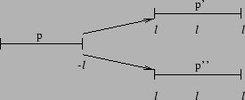
Conventional planning literature often speaks of clobbering and achieving preconditions of plans [Weld, 1994]. In CHiPs, these notions are slightly different since inconditions can clobber and be clobbered, as seen in the previous section. Formalizing these concepts and another, undoing postconditions, helps us define summary conditions (in Section 3.2). However, it will be convenient to define first what it means to assert a condition. Figure 5 gives examples of executions involved in these interactions, and we define these terms as follows:
Definition 2 states that an execution ![]() in a history
in a history ![]() asserts a literal at time
asserts a literal at time ![]() if that literal is an effect of
if that literal is an effect of ![]() that holds in the state at
that holds in the state at ![]() .
Note that that from this point on, beginning in Definition 3, we use
brackets [ ] as a shorthand when defining similar terms and procedures.
For example, saying ``[
.
Note that that from this point on, beginning in Definition 3, we use
brackets [ ] as a shorthand when defining similar terms and procedures.
For example, saying ``[![]() ,
, ![]() ] implies [
] implies [![]() ,
, ![]() ]'' means
]'' means ![]() implies
implies ![]() , and
, and ![]() implies
implies ![]() . This shorthand will help us avoid repetition,
at the cost of slightly more difficult parsing.
. This shorthand will help us avoid repetition,
at the cost of slightly more difficult parsing.
So, an execution achieves or clobbers a precondition if it is the last
(or one of the last) to assert the condition or its negation
(respectively) before it is required. Likewise, an execution undoes a postcondition if it is the first (or one of the first) to assert the negation of the condition after the condition is asserted. An execution ![]() clobbers an
incondition or postcondition of
clobbers an
incondition or postcondition of ![]() if
if ![]() asserts the negation of
the condition during or at the end (respectively) of
asserts the negation of
the condition during or at the end (respectively) of ![]() .
Achieving effects (inconditions and postconditions) does not make sense for this
formalism, so it is not defined.
Figure 5 shows different ways an execution
.
Achieving effects (inconditions and postconditions) does not make sense for this
formalism, so it is not defined.
Figure 5 shows different ways an execution ![]() achieves, clobbers, and undoes an execution
achieves, clobbers, and undoes an execution ![]() .
. ![]() and
and ![]() point to where they are asserted or required to be met.
point to where they are asserted or required to be met.
As recognized by tsuneto:98, external conditions are important
for reasoning about potential refinements of abstract plans. Although
the basic idea is the same, we define them a little differently and call
them external preconditions to differentiate them from other
conditions that we call external postconditions. Intuitively, an
external precondition of a group of partially ordered plans is a
precondition of one of the plans that is not achieved by another in
the group and must be met external to the group. External
postconditions, similarly, are those that are not undone by plans in
the group and are net effects of the group.
Definition 6 states that ![]() is an
external [pre, post]condition of an execution
is an
external [pre, post]condition of an execution ![]() if
if ![]() is a
[pre, post]condition of a subplan for which it is not [achieved,
undone] by some other subplan.
is a
[pre, post]condition of a subplan for which it is not [achieved,
undone] by some other subplan.
For the example in Figure 2, ![]() is not an external precondition because, although G must exist to produce H, G is supplied by the execution of the
is not an external precondition because, although G must exist to produce H, G is supplied by the execution of the
![]() plan. Thus,
plan. Thus, ![]() is met internally,
making
is met internally,
making ![]() an internal condition.
an internal condition.
![]() is an external precondition, an
internal condition, and an external postcondition because it is needed
externally and internally; it is an effect of
is an external precondition, an
internal condition, and an external postcondition because it is needed
externally and internally; it is an effect of ![]() which releases M1 when it is finished; and no other plan in the
decomposition undoes this effect.
which releases M1 when it is finished; and no other plan in the
decomposition undoes this effect.
Summary information can be used to find abstract solutions that are guaranteed to succeed no matter how they are refined because the information describes all potential conditions of the underlying decomposition. Thus, some commitments to particular plan choices, whether for a single agent or between agents, can be made based on summary information without worrying that deeper details lurk beneath that will doom the commitments. While HTN planners have used abstract conditions to guide search []<e.g.,>sacerdoti:74,tsuneto:98, they rely on a user-defined subset of constraints that can only help detect some potential conflicts. In contrast, summary information can be used to identify all potential conflicts.
Having the formalisms of the previous section, we can now define summary information and describe a method for computing it for non-primitive plans (in Section 3.4). Because there are many detailed definitions and algorithms in this section, we follow the same structure here as in the previous section, where we first give a more informal overview of the key concepts and notation, into which we then subsequently delve more systematically.
The
summary information of plan ![]() consists of summary pre-, in-, and
postconditions (
consists of summary pre-, in-, and
postconditions (![]() ,
, ![]() ,
, ![]() ),
summary resource usage (
),
summary resource usage (![]() ) for each resource
) for each resource ![]() ,
and whether the plan can be executed in any way successfully
(
,
and whether the plan can be executed in any way successfully
(![]() ).
).
A summary condition (whether pre, post, or in) specifies not only a positive
or negated literal, but additional modal information.
Each summary condition has an associated ![]() , whose value is either
, whose value is either ![]() or
or ![]() depending
on whether it must hold for all possible decompositions of the abstract operator
or just may hold depending on which decomposition is chosen. The
depending
on whether it must hold for all possible decompositions of the abstract operator
or just may hold depending on which decomposition is chosen. The
![]() of a summary condition is either
of a summary condition is either ![]() ,
, ![]() ,
, ![]() ,
or
,
or ![]() , specifying when the condition must hold in the plan's
interval of execution.
A plan
, specifying when the condition must hold in the plan's
interval of execution.
A plan ![]() must [achieve, clobber] summary
precondition
must [achieve, clobber] summary
precondition ![]() of
of ![]() if the execution of
if the execution of ![]() (or that of any plan with the same summary information) would [achieve, clobber] a condition summarized by
(or that of any plan with the same summary information) would [achieve, clobber] a condition summarized by ![]() (or any plan with the same summary information as
(or any plan with the same summary information as ![]() ).
).
The algorithm for deriving summary conditions for plan ![]() takes as
input the summary conditions of the immediate subplans of
takes as
input the summary conditions of the immediate subplans of ![]() and the
conditions defined for the CHiP
and the
conditions defined for the CHiP ![]() . The pre-, in-, and
postconditions of
. The pre-, in-, and
postconditions of ![]() become must first, must always, and must last
summary conditions, respectively. The algorithm retains the existence
and timing of subplan summary conditions in the parent depending on
whether the conditions are achieved, clobbered, or undone by siblings,
whether the decomposition is
become must first, must always, and must last
summary conditions, respectively. The algorithm retains the existence
and timing of subplan summary conditions in the parent depending on
whether the conditions are achieved, clobbered, or undone by siblings,
whether the decomposition is ![]() or
or ![]() , whether the subplan is
ordered first or last, and whether all subplans share the same
condition. Subplan first, always, and last conditions can become
sometimes conditions in the parent. The parent is computed as
, whether the subplan is
ordered first or last, and whether all subplans share the same
condition. Subplan first, always, and last conditions can become
sometimes conditions in the parent. The parent is computed as
![]() as long as all subplans are
as long as all subplans are ![]() , no subplan may
clobber a summary condition of another, and summarized resources do
not violate limits.
, no subplan may
clobber a summary condition of another, and summarized resources do
not violate limits.
We represent summary resource usage as three value ranges,
![]() ,
, ![]() ,
, ![]() ,
where the resource's local usage occurs within the task's execution,
and the persistent usage represents the usage that lasts after the
task terminates for depletable resources. The summarization algorithm
for an abstract task takes the summary resource usages of its
subtasks, considers all legal orderings of the subtasks, and all
possible usages for all subintervals within the interval of the
abstract task, to build multiple usage profiles. These profiles are
combined with algorithms for computing parallel, sequential, and
disjunctive usages to give the summary usage of the parent
task.
,
where the resource's local usage occurs within the task's execution,
and the persistent usage represents the usage that lasts after the
task terminates for depletable resources. The summarization algorithm
for an abstract task takes the summary resource usages of its
subtasks, considers all legal orderings of the subtasks, and all
possible usages for all subintervals within the interval of the
abstract task, to build multiple usage profiles. These profiles are
combined with algorithms for computing parallel, sequential, and
disjunctive usages to give the summary usage of the parent
task.
The summary information for a plan ![]() ,
, ![]() ,
is a tuple
,
is a tuple ![]() ,
, ![]() ,
, ![]() ,
, ![]() ,
, ![]() , whose
members are sets of summary conditions, summarized resource usage, and a
, whose
members are sets of summary conditions, summarized resource usage, and a ![]() flag indicating whether the plan will execute consistently internally.
flag indicating whether the plan will execute consistently internally.
![]() and
and
![]() are summary pre- and postconditions, which are the external pre- and postconditions of
are summary pre- and postconditions, which are the external pre- and postconditions of ![]() , respectively.
The summary inconditions of
, respectively.
The summary inconditions of ![]() ,
, ![]() , contain all
conditions that must hold within some execution of
, contain all
conditions that must hold within some execution of ![]() for it to be
successful. A condition
for it to be
successful. A condition ![]() in one of these sets is a tuple
in one of these sets is a tuple
![]() .
. ![]() is the literal of
is the literal of ![]() .
The
.
The ![]() of
of ![]() can be
can be ![]() or
or ![]() . If
. If
![]() , then
, then ![]() is called a
is called a ![]() condition because
condition because
![]() must hold for every successful plan execution.
For convenience we usually write
must hold for every successful plan execution.
For convenience we usually write ![]() .
. ![]() is a
is a ![]() condition (
condition (![]() is
is ![]() ) if
) if ![]() must hold for some successful execution.
must hold for some successful execution.
The ![]() of a summary condition
of a summary condition ![]() can
either be
can
either be ![]() ,
, ![]() ,
, ![]() , or
, or ![]() .
. ![]() is
is ![]() for
for ![]() if
if ![]() is an incondition that
must hold throughout all potential executions of
is an incondition that
must hold throughout all potential executions of ![]() (
(![]() holds
always); otherwise,
holds
always); otherwise, ![]() meaning
meaning ![]() holds at one point, at least, within an execution of
holds at one point, at least, within an execution of ![]() .
So, an
.
So, an ![]() condition is
condition is ![]() , and we do not define
, and we do not define ![]()
![]() inconditions because whether it is
inconditions because whether it is ![]() because of existence or timing, it is not significantly different from
because of existence or timing, it is not significantly different from ![]()
![]() in how a planner reasons about it. Whether a condition is
in how a planner reasons about it. Whether a condition is ![]()
![]() (however defined) or
(however defined) or ![]()
![]() , another plan can only have a
, another plan can only have a ![]()
![]() relationship with the condition (as defined in Section 3.3).
Note also that the incondition of a CHiP has the restricted meaning of a
relationship with the condition (as defined in Section 3.3).
Note also that the incondition of a CHiP has the restricted meaning of a ![]()
![]() summary incondition.
The
summary incondition.
The
![]() is
is ![]() for
for ![]() if
if ![]() holds at the
beginning of an execution of
holds at the
beginning of an execution of ![]() ; otherwise,
; otherwise, ![]() .
Similarly,
.
Similarly, ![]() is
is ![]() for
for ![]() if
if ![]() is
asserted at the end of a successful execution of
is
asserted at the end of a successful execution of ![]() ; otherwise, it is
; otherwise, it is ![]() .
Although
.
Although ![]() and
and ![]() syntactically only take one value,
semantically
syntactically only take one value,
semantically ![]() , and
, and ![]() .
.
We considered using modal logic operators to describe these concepts. While a mix of existing temporal logic and dynamic logic [Pratt, 1976] notation could be forced to work, we found that using our own terminology made definitions much simpler. We discuss this more at the end of Section 8.
Definitions 7, 8, and 9 give the formal semantics of ![]() and
and ![]() for a few representative condition types.
Summary conditions of a plan are defined recursively in that they
depend on the summary conditions of the plan's immediate subplans
instead of its complete decomposition.
Because a single description of summary information could represent
many different plan hierarchies, we quantify over plans
for a few representative condition types.
Summary conditions of a plan are defined recursively in that they
depend on the summary conditions of the plan's immediate subplans
instead of its complete decomposition.
Because a single description of summary information could represent
many different plan hierarchies, we quantify over plans ![]() , whose
subplans have the same summary information as those of the plan
, whose
subplans have the same summary information as those of the plan ![]() being summarized.
We could have defined the existence and timing
properties of conditions based on the entire hierarchy, but in doing
so, deriving summary conditions would be as expensive as solving the
planning problem, and one of the main purposes of summary information
is to reduce the computation of the planning problem. The reason why
it would be so expensive is that in the worst case all legal orderings of all plan steps must be explored to determine whether a
condition is
being summarized.
We could have defined the existence and timing
properties of conditions based on the entire hierarchy, but in doing
so, deriving summary conditions would be as expensive as solving the
planning problem, and one of the main purposes of summary information
is to reduce the computation of the planning problem. The reason why
it would be so expensive is that in the worst case all legal orderings of all plan steps must be explored to determine whether a
condition is ![]() or
or ![]() . We will discuss an example of this at the end of this subsection.
. We will discuss an example of this at the end of this subsection.
Definition 7 states that a ![]() precondition of
precondition of ![]() is an external
precondition that is always required at the beginning of the execution of any
is an external
precondition that is always required at the beginning of the execution of any
![]() that has the same conditions as
that has the same conditions as ![]() and the same summary information and ordering for its subplans as
and the same summary information and ordering for its subplans as ![]() .
A last postcondition is always asserted at the end of the execution
(substitute ``pre'' with ``post'' and
.
A last postcondition is always asserted at the end of the execution
(substitute ``pre'' with ``post'' and ![]() with
with ![]() in the last two lines of Definition 7). A
[must,may] sometimes precondition is a [must,may] external precondition
that is not a
in the last two lines of Definition 7). A
[must,may] sometimes precondition is a [must,may] external precondition
that is not a ![]() precondition. A sometimes postcondition
is defined similarly.
Definition 8 states that a literal
precondition. A sometimes postcondition
is defined similarly.
Definition 8 states that a literal ![]() is a
is a ![]() ,
, ![]() incondition of a plan
incondition of a plan ![]() if at any time during any isolated execution of any
if at any time during any isolated execution of any ![]() with the same summary information as
with the same summary information as ![]() , some executing plan
, some executing plan ![]() has incondition
has incondition ![]() .
Definition 9 states that a
[must, may] sometimes incondition of plan
.
Definition 9 states that a
[must, may] sometimes incondition of plan ![]() is a condition that is required during [any, some] execution of [any, some] plan
is a condition that is required during [any, some] execution of [any, some] plan ![]() that has the same summary information and ordering for its subplans as
that has the same summary information and ordering for its subplans as ![]() .
.
The ![]() flag is a boolean indicating whether the plan (or any
plan with the same summary information and ordering for subplans)
would execute successfully no matter how it was decomposed and no matter when
its subplans were executed. Definition 10 says that all
possible executions will succeed for a consistent plan. This is very similar to the
flag is a boolean indicating whether the plan (or any
plan with the same summary information and ordering for subplans)
would execute successfully no matter how it was decomposed and no matter when
its subplans were executed. Definition 10 says that all
possible executions will succeed for a consistent plan. This is very similar to the ![]() relation that will be defined in Section 4. We do not
include whether the plan will definitely not succeed in the summary
information because it requires an exponential computation to see whether
all conflicts in the subplans can be resolved. This computation can wait
to be done during planning after summary information is fully derived.
relation that will be defined in Section 4. We do not
include whether the plan will definitely not succeed in the summary
information because it requires an exponential computation to see whether
all conflicts in the subplans can be resolved. This computation can wait
to be done during planning after summary information is fully derived.
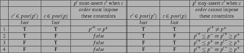
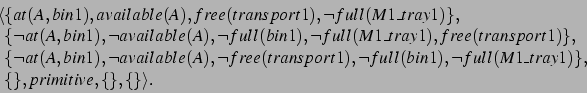
We show a subset of the summary conditions for
the production manager's top-level plan (of Figure 2) below.
Following each literal
are modal tags for ![]() and
and ![]() information. ``Mu'' is
information. ``Mu'' is
![]() ; ``Ma'' is
; ``Ma'' is ![]() ; ``F'' is
; ``F'' is ![]() ; ``L'' is
; ``L'' is ![]() ; ``S'' is
; ``S'' is
![]() ; and ``A'' is
; and ``A'' is ![]() .
.
Production manager's
The ![]() summary precondition is a
summary precondition is a ![]() condition
because the production manager may end up not using M1 if it chooses to use M2
instead to produce G.
condition
because the production manager may end up not using M1 if it chooses to use M2
instead to produce G. ![]() is a
is a ![]() summary
precondition because part A must be used at the beginning of execution
when it is transported to one of the machines.
Because the machines are needed sometime after the parts are transported, they are sometimes (and not first) conditions: they are needed at some point in time after the beginning of execution.
summary
precondition because part A must be used at the beginning of execution
when it is transported to one of the machines.
Because the machines are needed sometime after the parts are transported, they are sometimes (and not first) conditions: they are needed at some point in time after the beginning of execution.
Because the production manager may use M1 to produce G, ![]() is a summary
incondition of
is a summary
incondition of ![]() .
Having both
.
Having both ![]() and
and ![]() as inconditions
is consistent because they are
as inconditions
is consistent because they are ![]() conditions, implying that
they hold at different times during the plan's execution. In contrast, these
conditions would conflict if they were both
conditions, implying that
they hold at different times during the plan's execution. In contrast, these
conditions would conflict if they were both ![]() and
and ![]() (meaning that they must always hold throughout every possible execution of the plan).
(meaning that they must always hold throughout every possible execution of the plan).
The summary condition ![]() is a
is a ![]() postcondition of the top-level
plan because A will definitely be consumed by
postcondition of the top-level
plan because A will definitely be consumed by ![]() and is not
produced by some other plan in the decomposition of
and is not
produced by some other plan in the decomposition of
![]() . Even though
. Even though ![]() is an effect of
is an effect of
![]() , it is not an external postcondition of
, it is not an external postcondition of ![]() because it is undone by
because it is undone by ![]() , which consumes G to
make H.
, which consumes G to
make H. ![]() is a
is a ![]() summary postcondition because the
production manager releases H at the very end of execution.
summary postcondition because the
production manager releases H at the very end of execution.
![]() is not
is not ![]() because the manager finishes using M2
before moving H into storage.
because the manager finishes using M2
before moving H into storage.
Notice that ![]() is a
is a ![]() summary precondition. However,
no matter how the hierarchy is decomposed, M2 must be used to produce
H, so
summary precondition. However,
no matter how the hierarchy is decomposed, M2 must be used to produce
H, so ![]() must be established externally to the production
manager's plan. Because summary information is defined in terms of
the summary information of the immediate subplans, in the subplans of
must be established externally to the production
manager's plan. Because summary information is defined in terms of
the summary information of the immediate subplans, in the subplans of
![]() , we only see that
, we only see that ![]() has an
has an ![]() precondition and an
precondition and an ![]() postcondition that would
achieve the
postcondition that would
achieve the ![]() precondition of
precondition of ![]() .
This summary information does not tell us that the precondition of
.
This summary information does not tell us that the precondition of
![]() exists only when the postcondition exists, a necessary
condition to determine that the derived precondition of
exists only when the postcondition exists, a necessary
condition to determine that the derived precondition of ![]() is a
is a ![]() condition. Thus, it is
condition. Thus, it is ![]() . If we augmented summary
information with which subsets of conditions existed together, hunting
through combinations and temporal orderings of condition subsets among
subplans to derive summary conditions would basically be an
adaptation of an HTN planning algorithm, which summary information is
intended to improve. Instead, we derive summary information in
polynomial time and then use it to improve HTN planning exponentially
as we explain in Section 6.
This is the tradeoff we made at the beginning of this section in
defining summary conditions in terms of just the immediate subplans
instead of the entire hierarchy. Abstraction involves loss of
information, and this loss enables computational gains.
. If we augmented summary
information with which subsets of conditions existed together, hunting
through combinations and temporal orderings of condition subsets among
subplans to derive summary conditions would basically be an
adaptation of an HTN planning algorithm, which summary information is
intended to improve. Instead, we derive summary information in
polynomial time and then use it to improve HTN planning exponentially
as we explain in Section 6.
This is the tradeoff we made at the beginning of this section in
defining summary conditions in terms of just the immediate subplans
instead of the entire hierarchy. Abstraction involves loss of
information, and this loss enables computational gains.
In order to derive summary conditions according to their definitions, we need to be able to recognize achieve, clobber, and undo relationships based on summary conditions as we did for basic CHiP conditions. We give definitions and algorithms for these, which build on constructs and algorithms for reasoning about temporal relationships, described in Appendix A.
Achieving and clobbering are very similar, so we define them together.
Definition 11 states that plan ![]() must [achieve, clobber] summary
precondition
must [achieve, clobber] summary
precondition ![]() of
of ![]() if and only if for all executions of any
two plans,
if and only if for all executions of any
two plans, ![]() and
and ![]() , with the same summary information and
ordering constraints as
, with the same summary information and
ordering constraints as ![]() and
and ![]() , the execution of
, the execution of ![]() or
one of its subexecutions would [achieve, clobber] an external
precondition
or
one of its subexecutions would [achieve, clobber] an external
precondition ![]() of
of ![]() .
.
Achieving and clobbering in- and postconditions are defined the same as
Definition 11 but substituting ``in'' and ``post'' for ``pre'' and
removing the last line for inconditions. Additionally substituting
![]() for
for ![]() gives the definitions of may achieve
and clobber. Furthermore, the definitions of must/may-undo are
obtained by substituting ``post'' for ``pre'' and ``undo'' for
``achieve'' in Definition 11.
Note that, as mentioned in Section 2.5, achieving inconditions and
postconditions does not make sense for this formalism.
gives the definitions of may achieve
and clobber. Furthermore, the definitions of must/may-undo are
obtained by substituting ``post'' for ``pre'' and ``undo'' for
``achieve'' in Definition 11.
Note that, as mentioned in Section 2.5, achieving inconditions and
postconditions does not make sense for this formalism.
Algorithms for these interactions are given in
Figure 6 and Figure 7.
These algorithms build on others (detailed in Appendix B) that use interval point algebra to determine whether a plan must or
may assert a summary condition before, at, or during the time another
plan requires a summary condition to hold.
Similar to Definition 3 of must-achieve for CHiP conditions, Figure 6 says that ![]() achieves summary condition
achieves summary condition ![]() if it must asserts the condition before it must hold, and there are no other plans that may assert the condition or its negative in between.
The algorithm for may-achieve (in Figure 7) mainly differs in that
if it must asserts the condition before it must hold, and there are no other plans that may assert the condition or its negative in between.
The algorithm for may-achieve (in Figure 7) mainly differs in that ![]() may assert the condition beforehand, and there is no plan that must assert in between.
The undo algorithms are the same as those for achieve after swapping
may assert the condition beforehand, and there is no plan that must assert in between.
The undo algorithms are the same as those for achieve after swapping ![]() and
and ![]() in all
in all ![]() /
/![]() -
-![]() lines.
lines.
The complexity of determining must/may-clobber for inconditions and
postconditions is simply ![]() to check
to check ![]() conditions in
conditions in ![]() . If
the conditions are hashed, then the algorithm is constant time. For the
rest of the algorithm cases, the complexity of walking through the summary
conditions checking for
. If
the conditions are hashed, then the algorithm is constant time. For the
rest of the algorithm cases, the complexity of walking through the summary
conditions checking for ![]() and
and ![]() is
is ![]() for a maximum of
for a maximum of ![]() summary
conditions for each of
summary
conditions for each of ![]() plans represented in
plans represented in ![]() . In the
worst case, all summary conditions summarize the same propositional
variable, and all
. In the
worst case, all summary conditions summarize the same propositional
variable, and all ![]() conditions must be visited.
conditions must be visited.
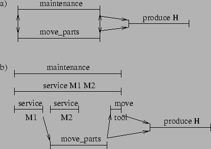
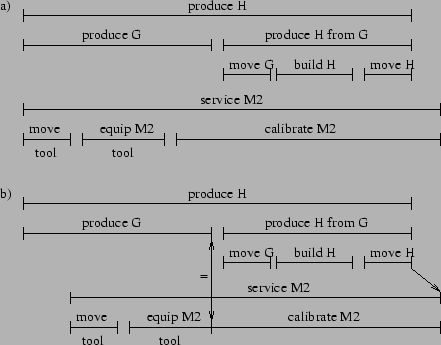
Let's look at some examples of these relationships.
In Figure 8a, ![]() may-clobber
may-clobber ![]() =
= ![]() (M2)MaS
in the summary
preconditions of
(M2)MaS
in the summary
preconditions of ![]() because there is some history
where
because there is some history
where ![]() ends before
ends before ![]() starts, and
starts, and
![]() starts after
starts after ![]() starts.
In Figure 8b,
starts.
In Figure 8b, ![]() must-achieve
must-achieve ![]() =
= ![]() (H)MuF in the summary
preconditions of
(H)MuF in the summary
preconditions of ![]() . Here,
. Here, ![]() is
is
![]() (H)MuL in the summary postconditions of
(H)MuL in the summary postconditions of ![]() . In all
histories,
. In all
histories, ![]() attempts to assert
attempts to assert ![]() before
the
before
the ![]() requires
requires ![]() to be met, and there is no
other plan execution that attempts to assert a condition on
the availability of H.
to be met, and there is no
other plan execution that attempts to assert a condition on
the availability of H. ![]() does not
may-clobber
does not
may-clobber ![]() =
= ![]() (M2)MuF in the
summary preconditions of
(M2)MuF in the
summary preconditions of ![]() even though
even though ![]() asserts
asserts ![]() =
= ![]() (M2)MuL before
(M2)MuL before ![]() is required to be met. This is because
is required to be met. This is because
![]() must assert
must assert ![]() (M2)MuA between the time that
(M2)MuA between the time that ![]() asserts
asserts ![]() and when
and when ![]() is required.
Thus,
is required.
Thus, ![]() must-undo
must-undo ![]() 's summary postcondition.
Because
's summary postcondition.
Because ![]() cannot assert its postcondition
cannot assert its postcondition
![]() (M2)MuL before
(M2)MuL before ![]() requires
requires
![]() (M2)MuF,
(M2)MuF, ![]() must-clobber the summary
precondition.
must-clobber the summary
precondition.
 |
Now that we have algorithms that determine interactions of abstract plans based on their summary conditions, we can create an algorithm that derives summary conditions according to their definitions in Section 3.2.
Figure 9 shows pseudocode for the algorithm.
The method for deriving the summary conditions of a plan ![]() is
recursive. First, summary information is derived for each of
is
recursive. First, summary information is derived for each of
![]() 's subplans. Then conditions are added based on
's subplans. Then conditions are added based on ![]() 's own conditions. Most of the rest of the algorithm
derives summary
conditions from those of
's own conditions. Most of the rest of the algorithm
derives summary
conditions from those of ![]() 's subplans.
Whether
's subplans.
Whether ![]() is
is ![]() depends on the consistency of its subplans and whether its own summary conditions and resource usages are in conflict. The braces '{' '}' used here have slightly different semantics than used before with the brackets. An expression {
depends on the consistency of its subplans and whether its own summary conditions and resource usages are in conflict. The braces '{' '}' used here have slightly different semantics than used before with the brackets. An expression {![]() ,
,![]() } can be interpreted simply as (
} can be interpreted simply as (![]() or
or ![]() , respectively).
, respectively).
Definitions and algorithms for temporal relationships such as ![]() -
-![]() and covers are in Appendix A.
When the algorithm adds or copies a condition to a set, only one condition can exist for any literal, so a condition's information may be overwritten if it has the same literal. In all cases,
and covers are in Appendix A.
When the algorithm adds or copies a condition to a set, only one condition can exist for any literal, so a condition's information may be overwritten if it has the same literal. In all cases, ![]() overwrites
overwrites ![]() ; and
; and ![]() ,
, ![]() , and
, and ![]() overwrite
overwrite ![]() ; but, not vice-versa.
Further, because it uses recursion, this procedure is assumed to work on plans whose expansion is finite.
; but, not vice-versa.
Further, because it uses recursion, this procedure is assumed to work on plans whose expansion is finite.
In this section, we
define a representation for capturing ranges of usage
both local to the task interval and the depleted usage lasting after
the end of the interval. Based on this we introduce a summarization
algorithm that captures in these ranges the uncertainty represented by
decomposition choices in ![]() plans and partial temporal orderings of
plans and partial temporal orderings of
![]() plan subtasks. This representation allows a coordinator or
planner to reason about the potential for conflicts for a set of tasks.
We will discuss this reasoning later in Section 4.2.
Although referred to as resources, these variables could be durations or
additive costs or rewards.
plan subtasks. This representation allows a coordinator or
planner to reason about the potential for conflicts for a set of tasks.
We will discuss this reasoning later in Section 4.2.
Although referred to as resources, these variables could be durations or
additive costs or rewards.
We start with a new example for simplicity that motivates our choice of representation. Consider the task of coordinating a collection of rovers as they explore the environment around a lander on Mars. This exploration takes the form of visiting different locations and making observations. Each traversal between locations follows established paths to minimize effort and risk. These paths combine to form a network like the one mapped out in Figure 10, where vertices denote distinguished locations, and edges denote allowed paths. Thinner edges are harder to traverse, and labeled points have associated observation goals. While some paths are over hard ground, others are over loose sand where traversal is harder since a rover can slip.
Figure 11 gives an example of an abstract task. Imagine a
rover that wants to make an early morning trip from point ![]() to point
to point
![]() on the example map. During this trip the sun slowly rises above
the horizon giving the rover the ability to progressively use soak rays tasks to provide more solar power (a non-consumable
resource3) to motors in the wheels. In addition to collecting photons,
the morning traverse moves the rover, and the resultant go tasks
require path dependent amounts of power. While a rover traveling from
point
on the example map. During this trip the sun slowly rises above
the horizon giving the rover the ability to progressively use soak rays tasks to provide more solar power (a non-consumable
resource3) to motors in the wheels. In addition to collecting photons,
the morning traverse moves the rover, and the resultant go tasks
require path dependent amounts of power. While a rover traveling from
point ![]() to point
to point ![]() can take any number of paths, the shortest
three involve following one, two, or three steps.
can take any number of paths, the shortest
three involve following one, two, or three steps.
A summarized resource usage consists of
ranges of potential resource usage amounts during
and after performing an abstract task, and we represent this
summary information for a plan ![]() on a resource
on a resource ![]() using the structure
using the structure
![]() where the resource's local usage occurs within
where the resource's local usage occurs within ![]() 's
execution, and the persistent usage represents the usage that lasts
after the execution terminates for consumable resources.
's
execution, and the persistent usage represents the usage that lasts
after the execution terminates for consumable resources.
The context for Definition 12 is the set of all
histories ![]() where the value of
where the value of ![]() is 0 in the initial state, and
is 0 in the initial state, and
![]() only contains the execution of
only contains the execution of ![]() and its subexecutions. Thus,
the
and its subexecutions. Thus,
the ![]() term is the combined usage of
term is the combined usage of ![]() at time
at time ![]() of all
executions in the hierarchy as defined in Section 2.4.
So, the maximum of the
of all
executions in the hierarchy as defined in Section 2.4.
So, the maximum of the ![]() is the highest among all
histories of the lowest point of usage during
is the highest among all
histories of the lowest point of usage during ![]() 's execution.
The usage ranges capture the multiple possible usage profiles of a
task with multiple decomposition choices and timing choices among
loosely constrained subtasks. For example, the high path task
has a
's execution.
The usage ranges capture the multiple possible usage profiles of a
task with multiple decomposition choices and timing choices among
loosely constrained subtasks. For example, the high path task
has a ![]() [4,4],[6,6],[0,0]
[4,4],[6,6],[0,0]![]() summary power use over a 40
minute interval. In this case the ranges are single points due to no
uncertainty - the task simply uses 4 watts for 15 minutes followed by
6 watts for 25 minutes. The
summary power use over a 40
minute interval. In this case the ranges are single points due to no
uncertainty - the task simply uses 4 watts for 15 minutes followed by
6 watts for 25 minutes. The ![]() (A,B) task provides a slightly more
complex example due to its decompositional uncertainty. This task has
a
(A,B) task provides a slightly more
complex example due to its decompositional uncertainty. This task has
a ![]() [0,4],[4,6],[0,0]
[0,4],[4,6],[0,0]![]() summary power use over a 50 minute
interval. In both cases the
summary power use over a 50 minute
interval. In both cases the ![]() is [0,0] because solar
power is a non-consumable resource.
is [0,0] because solar
power is a non-consumable resource.
As an example of
reasoning with resource usage summaries, suppose that only 3 watts of
power were available during a ![]() (A,B) task. Given the [4,6]
(A,B) task. Given the [4,6]
![]() , we know that there is not enough power no matter
how the task is decomposed. Raising the available power to 4 watts
makes the task executable depending on how it gets decomposed and
scheduled, and raising to 6 or more watts makes the task executable
for all possible decompositions.
, we know that there is not enough power no matter
how the task is decomposed. Raising the available power to 4 watts
makes the task executable depending on how it gets decomposed and
scheduled, and raising to 6 or more watts makes the task executable
for all possible decompositions.
This representation of abstract (or uncertain) metric resource usage can be seen as an extension of tracking optimistic and pessimistic resource levels [Drabble Tate, 1994]. Computing only the upper and lower bounds on resource usage for an abstract plan gives some information about whether lower or upper bound constraints on a resource may, must, or must not be violated, but it is not complete. By representing upper and lower bounds as ranges of these bounds over all potential histories, we can certainly know whether bounds may, must, or must not be violated over all histories. For the example above, if we only tracked one range for the local usage, [0,6], we would not know that there is definitely a conflict when only 3 watts are available. Knowing this extra information can avoid exploration of an infeasible search space.
The state summarization algorithm in Section 3.4 recursively
propagates summary conditions upwards from an ![]() /
/![]() hierarchy's leaves,
and the algorithm for resource summarization takes the same approach.
Starting at the leaves, the algorithm finds primitive tasks that use constant
amounts of a resource. The resource summary of a task using
hierarchy's leaves,
and the algorithm for resource summarization takes the same approach.
Starting at the leaves, the algorithm finds primitive tasks that use constant
amounts of a resource. The resource summary of a task using
![]() units of a resource is
units of a resource is ![]() ,
,![]() ,
,![]() ,
,![]() ,
,![]() ,
,![]() or
or ![]() ,
,![]() ,
,![]() ,
,![]() ,
,![]() ,
,![]() over the task's duration for
non-consumable or consumable resources respectively.
over the task's duration for
non-consumable or consumable resources respectively.
Moving up the ![]() /
/![]() tree, the summarization algorithm either comes to
an
tree, the summarization algorithm either comes to
an ![]() or an
or an ![]() branch. For an
branch. For an ![]() branch the combined summary usage
comes from the
branch the combined summary usage
comes from the ![]() computation
computation
![\begin{displaymath}
\setlength{\arraycolsep}{0in}
\begin{array}[t]{lllll}
\lang...
... & max_{c \in children}(ub(persist(c)))]&\ \rangle,
\end{array}\end{displaymath}](img223.png) where
where ![]() and
and ![]() extract the lower bound and upper bound of a
range respectively. The
extract the lower bound and upper bound of a
range respectively. The ![]() denote the branch's children with
their durations extended to the length of the longest child. This
duration extension alters a child's resource summary information
because the child's usage profile has a zero resource usage during the
extension. For instance, in determining the resource usage for
denote the branch's children with
their durations extended to the length of the longest child. This
duration extension alters a child's resource summary information
because the child's usage profile has a zero resource usage during the
extension. For instance, in determining the resource usage for
![]() (A,B), the algorithm combines two 40 minute tasks with a 50
minute task. The resulting summary information describes a 50 minute
abstract task whose profile might have a zero watt power usage for 10
minutes. This extension is why
(A,B), the algorithm combines two 40 minute tasks with a 50
minute task. The resulting summary information describes a 50 minute
abstract task whose profile might have a zero watt power usage for 10
minutes. This extension is why ![]() (A,B) has a [0,4] for a
(A,B) has a [0,4] for a
![]() instead of [3,4]. Planners that reason about
variable durations could use [3,4] for a duration ranging from 40 to
50.
instead of [3,4]. Planners that reason about
variable durations could use [3,4] for a duration ranging from 40 to
50.
Computing an ![]() branch's summary information is a bit more
complicated due to timing choices among loosely constrained subtasks.
The take
branch's summary information is a bit more
complicated due to timing choices among loosely constrained subtasks.
The take ![]() path examples illustrate the simplest sub-case,
where subtasks are tightly constrained to execute serially. Here
profiles are appended together, and the resulting summary usage
information comes from the SERIAL-AND computation
path examples illustrate the simplest sub-case,
where subtasks are tightly constrained to execute serially. Here
profiles are appended together, and the resulting summary usage
information comes from the SERIAL-AND computation
![\begin{displaymath}
\setlength{\arraycolsep}{0in}
\begin{array}[t]{lllll}
\lang...
...a_{c \in children}(ub(persist(c)))] & \ \rangle,\\
\end{array}\end{displaymath}](img227.png) where
where ![]() and
and ![]() are the
respective lower and upper bounds on the cumulative persistent usages
of children that execute before
are the
respective lower and upper bounds on the cumulative persistent usages
of children that execute before ![]() . These computations have the same
form as the
. These computations have the same
form as the ![]() computations for the final
computations for the final ![]() .
.
The case where all subtasks execute in parallel and have identical
durations is slightly simpler. Here the usage profiles add together,
and the branch's resultant summary usage comes from the PARALLEL-AND
computation
![\begin{displaymath}
\setlength{\arraycolsep}{0in}
\begin{array}[t]{lllll}
\lang...
...a_{c \in children}(ub(persist(c)))] & \ \rangle,\\
\end{array}\end{displaymath}](img231.png) where
where ![]() and
and ![]() are the
respective sums of the
are the
respective sums of the ![]() upper bounds and
the
upper bounds and
the ![]() lower bounds for all children except
lower bounds for all children except ![]() .
.
To handle ![]() tasks with loose temporal constraints, we consider all
legal orderings of child task endpoints. For example, in the rover's
early morning tasks, there are three serial solar energy collection
subtasks running in parallel with a subtask to drive to location
tasks with loose temporal constraints, we consider all
legal orderings of child task endpoints. For example, in the rover's
early morning tasks, there are three serial solar energy collection
subtasks running in parallel with a subtask to drive to location ![]() .
Figure 12 shows one possible ordering of the subtask
endpoints, which breaks
.
Figure 12 shows one possible ordering of the subtask
endpoints, which breaks ![]() (A,B) into three pieces, and two of
the soak rays children in half. Given an ordering, the
summarization algorithm can (1) use the endpoints of the children to
determine subintervals, (2) compute summary information for each child
task/subinterval combination, (3) combine the parallel subinterval
summaries using the PARALLEL-AND computation, and then (4) chain the
subintervals together using the SERIAL-AND computation. Finally, the
(A,B) into three pieces, and two of
the soak rays children in half. Given an ordering, the
summarization algorithm can (1) use the endpoints of the children to
determine subintervals, (2) compute summary information for each child
task/subinterval combination, (3) combine the parallel subinterval
summaries using the PARALLEL-AND computation, and then (4) chain the
subintervals together using the SERIAL-AND computation. Finally, the
![]() task's summary is computed by combining the summaries for all
possible orderings using an
task's summary is computed by combining the summaries for all
possible orderings using an ![]() computation.
computation.
Here we describe how step (2) generates different summary resource
usages for the subintervals of a child task.
A child task with summary resource usage
![]() ,
,![]() ,
,![]() ,
,![]() ,
,![]() ,
,![]() contributes one of two summary
resource usages to each intersecting subinterval4:
contributes one of two summary
resource usages to each intersecting subinterval4:
![]() While the first usage has the tighter [
While the first usage has the tighter [![]() ,
,![]() ],[
],[![]() ,
,![]() ] local ranges, the
second has looser [
] local ranges, the
second has looser [![]() ,
,![]() ],[
],[![]() ,
,![]() ] local ranges. Since the
] local ranges. Since the ![]() and
and ![]() bounds only apply to the subintervals containing the subtask's minimum
and maximum usages, the tighter ranges apply to one of a subtask's
intersecting subintervals. While the minimum and maximum usages may
not occur in the same subinterval, symmetry arguments let us connect
them in the computation. Thus one subinterval has tighter local
ranges and all other intersecting subintervals get the looser local
ranges, and the extra complexity comes from having to investigate all
subtask/subinterval assignment options. For instance, there are three
subintervals intersecting
bounds only apply to the subintervals containing the subtask's minimum
and maximum usages, the tighter ranges apply to one of a subtask's
intersecting subintervals. While the minimum and maximum usages may
not occur in the same subinterval, symmetry arguments let us connect
them in the computation. Thus one subinterval has tighter local
ranges and all other intersecting subintervals get the looser local
ranges, and the extra complexity comes from having to investigate all
subtask/subinterval assignment options. For instance, there are three
subintervals intersecting ![]() (A,B) in Figure 12,
and three different assignments of summary resource usages to the
subintervals: placing [0,4],[4,6] in one subinterval with
[0,6],[0,6] in the other two. These placement options result in a
subtask with
(A,B) in Figure 12,
and three different assignments of summary resource usages to the
subintervals: placing [0,4],[4,6] in one subinterval with
[0,6],[0,6] in the other two. These placement options result in a
subtask with ![]() subintervals having
subintervals having ![]() possible subinterval
assignments. So if there are
possible subinterval
assignments. So if there are ![]() child tasks each with
child tasks each with ![]() alternate
assignments, then there are
alternate
assignments, then there are ![]() combinations of potential
subtask/subinterval summary resource usage assignments. Thus
propagating summary information through an
combinations of potential
subtask/subinterval summary resource usage assignments. Thus
propagating summary information through an ![]() branch is exponential
in the number of subtasks with multiple internal subintervals.
However since the number of subtasks is controlled by the domain
modeler and is usually bounded by a constant, this computation is
tractable. In addition, summary information can often be derived
offline for a domain. The propagation algorithm takes on the form:
branch is exponential
in the number of subtasks with multiple internal subintervals.
However since the number of subtasks is controlled by the domain
modeler and is usually bounded by a constant, this computation is
tractable. In addition, summary information can often be derived
offline for a domain. The propagation algorithm takes on the form:
Now that we have described how to derive summary information, we can discuss how to use it.
Up to this point, we have detailed algorithms for
deriving summary conditions and for reasoning about potential (![]() )
and definite (
)
and definite (![]() ) interactions between tasks
based on their summary information. In addition, we
have outlined algorithms for deriving summarized resource usage but
have not yet discussed how to identify solutions at abstract levels.
In this section, we show how the interactions of summary conditions
and summarized metric resource usages identify potentially resolvable
threats and unresolvable conflicts among the plans of a group
of agents.
) interactions between tasks
based on their summary information. In addition, we
have outlined algorithms for deriving summarized resource usage but
have not yet discussed how to identify solutions at abstract levels.
In this section, we show how the interactions of summary conditions
and summarized metric resource usages identify potentially resolvable
threats and unresolvable conflicts among the plans of a group
of agents.
Agents can attempt to resolve conflicts among their plans by considering commitments to particular decompositions and ordering constraints. In order to do this, the agents must be able to identify remaining conflicts (threats) among their plans. Here we present simple algorithms for reasoning about threats between abstract plans and their required conditions.
Formally, for a set of CHiPs ![]() with ordering constraints
with ordering constraints ![]() , a
threat between an abstract plan
, a
threat between an abstract plan ![]() and a summary
condition
and a summary
condition ![]() of another plan
of another plan ![]() exists iff
exists iff ![]() may-clobber
may-clobber
![]() . We say that the threat is unresolvable if
. We say that the threat is unresolvable if ![]() must-clobber
must-clobber ![]() and
and
![]() because there are no decomposition choices or ordering constraints that could be added to resolve the threat.
because there are no decomposition choices or ordering constraints that could be added to resolve the threat.
So, a simple algorithm for identifying threats is to check to see if
each of the ![]() summary conditions of
summary conditions of ![]() plans in
plans in ![]() is
must- or may-clobbered by any other plan. Since the complexity of
checking to see if a particular condition is must- or may-clobbered is
is
must- or may-clobbered by any other plan. Since the complexity of
checking to see if a particular condition is must- or may-clobbered is
![]() , this algorithm's complexity is
, this algorithm's complexity is ![]() .
.
In many coordination tasks, if agents could determine that under
certain temporal constraints their plans can be decomposed in any way
(![]() ) or that under those constraints there is no way they can
be successfully decomposed (
) or that under those constraints there is no way they can
be successfully decomposed (![]() ), then they can make
coordination decisions at abstract levels without entering a
potentially costly search for valid plan merges at lower levels.
Here are the formal definitions of
), then they can make
coordination decisions at abstract levels without entering a
potentially costly search for valid plan merges at lower levels.
Here are the formal definitions of ![]() and
and ![]() :
:
Definition 13 states that the plans with summary
information ![]() under ordering constraints can execute in any
way if and only if all sets of plans
under ordering constraints can execute in any
way if and only if all sets of plans ![]() that have summary information
that have summary information
![]() will execute successfully in any history.
will execute successfully in any history. ![]() is true if
there is some set of plans that could possibly execute successfully.
We could also describe
is true if
there is some set of plans that could possibly execute successfully.
We could also describe ![]() ,
,![]() and
and ![]() ,
,![]() in the same fashion, but it is not obvious how their addition could further influence search. Exploring these relations may be an interesting topic for future research.
in the same fashion, but it is not obvious how their addition could further influence search. Exploring these relations may be an interesting topic for future research.
In Figure 13a, the three top-level plans of
the managers are unordered with respect to each other. The leaf plans
of the partially expanded hierarchies comprise ![]() . Arrows
represent the constraints in
. Arrows
represent the constraints in ![]() .
. ![]() ({},{
({},{![]() ,
,
![]() ,
, ![]() }) is false because there are several
conflicts over the use of machines and transports that could occur for
certain executions of the plans as described in Section
3.3 for Figure
8. However,
}) is false because there are several
conflicts over the use of machines and transports that could occur for
certain executions of the plans as described in Section
3.3 for Figure
8. However, ![]() ({}, {
({}, {![]() ,
, ![]() ,
,
![]() }) is true because the plans might in some way execute
successfully as shown in Figure 13b. With the ordering
constraints in Figure 13b,
}) is true because the plans might in some way execute
successfully as shown in Figure 13b. With the ordering
constraints in Figure 13b, ![]() ({before(1,0),
before(0,2)},{
({before(1,0),
before(0,2)},{![]() ,
, ![]() ,
, ![]() }) is true
because the plans can execute in any way consistent with these ordering constraints without conflict.
Figure 8b is an example where
}) is true
because the plans can execute in any way consistent with these ordering constraints without conflict.
Figure 8b is an example where ![]() is false because
is false because
![]() must-clobber the
must-clobber the ![]() (M2)MuF
summary precondition of
(M2)MuF
summary precondition of ![]() .
.
 |
As shown in Figure 14, the algorithm for determining
![]() for summary conditions is simple in that it only needs to check for threats.
for summary conditions is simple in that it only needs to check for threats.
![]() is more complicated because just checking for
an unresolvable threat is not enough. As shown in Figure
15, it is not the case that plan
is more complicated because just checking for
an unresolvable threat is not enough. As shown in Figure
15, it is not the case that plan ![]() must clobber
must clobber
![]() because
because ![]() could come between and achieve the precondition
could come between and achieve the precondition
![]() of
of ![]() . Thus,
. Thus, ![]() may-clobbers
may-clobbers ![]() in
in ![]() and in
and in ![]() .
However, obviously
.
However, obviously ![]() will clobber one or the other, so
will clobber one or the other, so
![]() is false. In order to determine
is false. In order to determine ![]() is
is
![]() , an agent must exhaustively search through an exponential number of schedules
to see if not all conflicts can be resolved. Instead of
performing an exponential search to determine
, an agent must exhaustively search through an exponential number of schedules
to see if not all conflicts can be resolved. Instead of
performing an exponential search to determine ![]() , we use the simple
algorithm in Figure 14 that just checks for
must-clobber relationships. In Section 5.1 we describe
a more flexible search to find conflict-free abstract plans than just
scheduling at an abstract level.
, we use the simple
algorithm in Figure 14 that just checks for
must-clobber relationships. In Section 5.1 we describe
a more flexible search to find conflict-free abstract plans than just
scheduling at an abstract level.
Thus, while the ![]() algorithm is sound and complete, the
algorithm is sound and complete, the
![]() algorithm is complete but not sound. This also means that determining
algorithm is complete but not sound. This also means that determining ![]() is sound but not complete. We will still
make use of both of these algorithms in a sound and complete
planning/coordination algorithm in Section 5.1.
The complexity of these algorithms
is
is sound but not complete. We will still
make use of both of these algorithms in a sound and complete
planning/coordination algorithm in Section 5.1.
The complexity of these algorithms
is ![]() since the
since the ![]() procedures for determining
must/may-clobber must be run for each of
procedures for determining
must/may-clobber must be run for each of ![]() conditions (
conditions (![]() summary conditions in each of
summary conditions in each of ![]() plans represented by
plans represented by ![]() ).
).
Planners detect threats on resource constraints in different ways. If the planner reasons about partially ordered actions, it must consider which combinations of actions can overlap and together exceed (or fall below) the resource's maximum value (or minimum value). A polynomial algorithm does this for the IxTeT planner [Laborie Ghallab, 1995]. Other planners that consider total order plans can more simply project the levels of the resource from the initial state through the plan, summing overlapping usages, to see if there are conflicts []<e.g.,>rabideau:00.
Finding conflicts involving summarized resource usages can work in the
same way. For the partial order planner, the resultant usage of
clusters of actions are tested using the PARALLEL-AND algorithm in
Section 3.5. For the total order planner, the level of
the resource is represented as a summarized usage, initially
![]() [
[![]() ,
, ![]() ], [
], [![]() ,
, ![]() ], [
], [![]() ,
, ![]() ]
]![]() for a consumable
resource with an initial level
for a consumable
resource with an initial level ![]() and
and ![]() [
[![]() ,
, ![]() ], [
], [![]() ,
,
![]() ], [0, 0]
], [0, 0]![]() for a non-consumable resource. Then, for each
subinterval between start and end times of the schedule of tasks, the
summary usage for each is computed using the PARALLEL-AND algorithm.
Then the level of the resource is computed for each subinterval while
propagating persistent usages using the SERIAL-AND algorithm.
for a non-consumable resource. Then, for each
subinterval between start and end times of the schedule of tasks, the
summary usage for each is computed using the PARALLEL-AND algorithm.
Then the level of the resource is computed for each subinterval while
propagating persistent usages using the SERIAL-AND algorithm.
We can decide ![]() and
and ![]() as defined in Section
4.1, in terms of the summary usage values resulting
from invocations of PARALLEL-AND and SERIAL-AND in the propagation algorithm at the end of Section 3.5.2.
as defined in Section
4.1, in terms of the summary usage values resulting
from invocations of PARALLEL-AND and SERIAL-AND in the propagation algorithm at the end of Section 3.5.2. ![]() is true if and only if there are no potential threats. These algorithms discover a threat if they ever compute an interval
is true if and only if there are no potential threats. These algorithms discover a threat if they ever compute an interval ![]() such that
such that
![\begin{displaymath}
\setlength{\arraycolsep}{0in}
\begin{array}[t]{lllll}
lb(lo...
...alue(res)\ \vee \ ub(persist(i)) > max\_value(res).
\end{array}\end{displaymath}](img264.png)
![]() is true if and only if there is a possible run with potentially no threats. SERIAL-AND discovers such a run if it returns a summary usage where
is true if and only if there is a possible run with potentially no threats. SERIAL-AND discovers such a run if it returns a summary usage where
![\begin{displaymath}
\setlength{\arraycolsep}{0in}
\begin{array}[t]{lllll}
ub(lo...
...res)\ \wedge \ ub(persist(i)) \leq max\_value(res).
\end{array}\end{displaymath}](img266.png)
Now that we have mechanisms for deriving summary information and evaluating plans based on their summarizations, we will discuss how to exploit them in a planning/coordination algorithm.
With the earlier defined algorithms for reasoning about a group of agents' plans at multiple levels of abstraction, we now describe how agents can efficiently plan and coordinate based on summary information. We describe a coordination algorithm that searches for ways to restrict the decomposition and ordering of the collective actions of the agent(s) in order to resolve conflicts while maximizing the utilities of the individual agents or the global utility of the group.
Our approach starts by making planning decisions at the most abstract level and, as needed, decomposes the agents' plans in a top-down fashion. The idea is to introduce only the information that is needed. Introducing irrelevant details complicates search and increases communication. After describing the top-down planning/coordination algorithm, we describe search techniques and heuristics that the algorithm can use to further exploit summary information.
The formalism of summary conditions culminated in Section 4 in algorithms
that determine if a set of plans (abstract or primitive)
under a partial set of ordering constraints is definitely conflict-free
(![]() ) or has unresolvable conflicts (
) or has unresolvable conflicts (![]() ).
Here we integrate these
algorithms into one
that searches for a consistent plan for one or more
agents.
The particular algorithm we describe here is shown to be sound and complete [Clement, 2002]. The
search starts out with the top-level plans of each agent. A solution is one where there are no possible conflicts among the agents' plans.
The algorithm tries to find a
solution at this top level and then expands the hierarchies deeper and
deeper until the optimal solution is found or the search space has
been exhausted. A pseudocode description of the algorithm is given in
Figure 16.
).
Here we integrate these
algorithms into one
that searches for a consistent plan for one or more
agents.
The particular algorithm we describe here is shown to be sound and complete [Clement, 2002]. The
search starts out with the top-level plans of each agent. A solution is one where there are no possible conflicts among the agents' plans.
The algorithm tries to find a
solution at this top level and then expands the hierarchies deeper and
deeper until the optimal solution is found or the search space has
been exhausted. A pseudocode description of the algorithm is given in
Figure 16.
A state of the search is a partially elaborated plan that we
represent as a set of ![]() plans (one for each agent), a set of
temporal constraints, and a set of blocked plans. The subplans of the
plans (one for each agent), a set of
temporal constraints, and a set of blocked plans. The subplans of the
![]() plans are the leaves of the partially expanded hierarchies of
the agents. The set of temporal constraints includes synchronization
constraints added during the search in addition to those dictated by
the agents' individual hierarchical plans. Blocked subplans keep
track of pruned
plans are the leaves of the partially expanded hierarchies of
the agents. The set of temporal constraints includes synchronization
constraints added during the search in addition to those dictated by
the agents' individual hierarchical plans. Blocked subplans keep
track of pruned ![]() subplans.
subplans.
Decisions can be made during search in a decentralized fashion. The agents can negotiate over ordering constraints to adopt, over choices of subplans to accomplish higher level plans, and over which decompositions to explore first. While the algorithm described here does not specify (or commit to) any negotiation technique, it does provide the mechanisms for identifying the choices over which the agents can negotiate. Although agents can make search decisions in a decentralized fashion, we describe the algorithm given here as a centralized process that requests summary information from the agents being coordinated.
In the pseudocode in Figure 16, the coordinating agent
collects summary information about the other agents' plans as it
decomposes them. The ![]() keeps track of expanded search states.
If the
keeps track of expanded search states.
If the ![]() relation holds for the search state, the Dominates function determines if the current solutions are better for
every agent than the solution represented by the current search state
and keeps it if the solution is not dominated. If
relation holds for the search state, the Dominates function determines if the current solutions are better for
every agent than the solution represented by the current search state
and keeps it if the solution is not dominated. If ![]() is
false, then the search space rooted at the current search state
can be pruned; otherwise, the coordinator applies operators to
generate new search states.
is
false, then the search space rooted at the current search state
can be pruned; otherwise, the coordinator applies operators to
generate new search states.
The operators for generating successor search states are expanding non-primitive plans,
blocking ![]() subplans, and adding temporal constraints on pairs of
plans. When an agent expands one of its plans, each of the plan's summary
conditions are replaced with only the original conditions of the
parent plan. Then the subplans' summary information and ordering constraints are
added to the search state.
A subplan of an
subplans, and adding temporal constraints on pairs of
plans. When an agent expands one of its plans, each of the plan's summary
conditions are replaced with only the original conditions of the
parent plan. Then the subplans' summary information and ordering constraints are
added to the search state.
A subplan of an ![]() plan is added (or selected) only when all
other subplans are blocked.
When ApplyOperator is called for the select and block operators, search states are generated for each selectable and blockable subplan, respectively.
Blocking an
plan is added (or selected) only when all
other subplans are blocked.
When ApplyOperator is called for the select and block operators, search states are generated for each selectable and blockable subplan, respectively.
Blocking an ![]() subplan can be effective
in resolving a constraint in which the other
subplan can be effective
in resolving a constraint in which the other ![]() subplans are not
involved. For example, if the inventory manager plans to only use transport2,
the production manager could block subplans using transport2, leaving subplans
using transport1 that do not conflict with the inventory manager's plan.
This can lead to least commitment abstract solutions that
leave the agents flexibility in selecting among the multiple
applicable remaining subplans. The agents can take another approach
by selecting a subplan (effectively blocking all of the others) to
investigate a preferred choice or one that more
likely avoids conflicts.
subplans are not
involved. For example, if the inventory manager plans to only use transport2,
the production manager could block subplans using transport2, leaving subplans
using transport1 that do not conflict with the inventory manager's plan.
This can lead to least commitment abstract solutions that
leave the agents flexibility in selecting among the multiple
applicable remaining subplans. The agents can take another approach
by selecting a subplan (effectively blocking all of the others) to
investigate a preferred choice or one that more
likely avoids conflicts.
When the operator is to add a temporal constraint, a new search state is created for each alternative temporal constraint that could be added. These successor states are enqueued so that if backtracking is needed, each alternative can be tried. Adding temporal constraints should only generate new search states when the ordering is consistent with the other global and local constraints. In our implementation, we only add constraints that will help resolve threats as determined by the must/may achieves and clobbers algorithms. When a plan is expanded or selected, the ordering constraints must be updated for the subplans that are added.
The soundness and completeness of the coordination algorithm depends on the soundness and completeness of identifying solutions and the complete exploration of the search space. Soundness and completeness is not defined with respect to achieving particular goal predicates but resolving conflicts in the plan hierarchies. A domain modeler may represent goals as abstract CHiPs that decompose into possible plans that accomplish them or as a series of actions for an agent to execute successfully.
Consider how the algorithm would find coordinated plans for the
manufacturing agents. At the beginning of the search, a coordinating agent
gathers the summary information for the top-level plans of the three
agents in ![]() . At first, there are no ordering constraints, so
. At first, there are no ordering constraints, so
![]() is empty in the first search state (shown in Figure
13a) popped from the
is empty in the first search state (shown in Figure
13a) popped from the ![]() .
. ![]() is false,
and
is false,
and ![]() is true for this state as described earlier in this
section, so the coordinator chooses an
is true for this state as described earlier in this
section, so the coordinator chooses an ![]() to apply to the
search state. It could choose constrain and order the
to apply to the
search state. It could choose constrain and order the
![]() plan before
plan before ![]() to resolve all conflicts
between those two plans.
The
to resolve all conflicts
between those two plans.
The
![]() is updated with the new constraint, and the new search state
is inserted into the
is updated with the new constraint, and the new search state
is inserted into the ![]() by according to some ranking function.
On the
next iteration of the loop, the only search state in the queue
that was just inserted is popped. The coordinator again finds that
by according to some ranking function.
On the
next iteration of the loop, the only search state in the queue
that was just inserted is popped. The coordinator again finds that
![]() is false, and
is false, and ![]() is true since
is true since ![]() may still conflict with other plans over the use of transports. It can
choose to constrain
may still conflict with other plans over the use of transports. It can
choose to constrain ![]() before
before ![]() to resolve the
remaining conflicts. This is detected on the next cycle of the search
loop where
to resolve the
remaining conflicts. This is detected on the next cycle of the search
loop where ![]() is found to be true for this search state
(shown in Figure 13b). The
is found to be true for this search state
(shown in Figure 13b). The ![]() , the two constraints
in
, the two constraints
in ![]() , and the empty set of blocked plans are added as a solution
since there is no previously found solution that Dominates it.
The Dominates function uses domain specific criteria for
determining when a solution has value as an alternative and should be
kept or is inferior compared to another and should be dropped. In
this manufacturing domain, one solution dominates another if the finish time
for at least one agent is earlier and no finish times are later for any agents. The search then
continues to find alternative or superior solutions, although the
agents may decide to terminate the search in the interest of time.
, and the empty set of blocked plans are added as a solution
since there is no previously found solution that Dominates it.
The Dominates function uses domain specific criteria for
determining when a solution has value as an alternative and should be
kept or is inferior compared to another and should be dropped. In
this manufacturing domain, one solution dominates another if the finish time
for at least one agent is earlier and no finish times are later for any agents. The search then
continues to find alternative or superior solutions, although the
agents may decide to terminate the search in the interest of time.
Although summary information is valuable for finding conflict free or
coordinated plans at abstract levels, this information can also be
valuable in directing the search to avoid branches in the search space
that lead to inconsistent or suboptimal coordinated plans. A coordinator can prune away inconsistent
coordinated plans at the abstract level by doing a quick
check to see if ![]() is false.
For example,
if the search somehow reached the state shown in Figure
8b, the coordinator could backtrack before
expanding the hierarchies further and avoid reasoning about details of
the plans where they must fail.
is false.
For example,
if the search somehow reached the state shown in Figure
8b, the coordinator could backtrack before
expanding the hierarchies further and avoid reasoning about details of
the plans where they must fail.
Another strategy is to first expand plans involved in the most
threats. For the sake of completeness, the order of plan expansions
does not matter as long as they are all expanded at some point when
the search trail cannot be pruned. But, employing this ``expand on
most threats first'' (EMTF) heuristic aims at driving the search down
through the hierarchy to find the subplan(s) causing conflicts with
others so that they can be resolved more quickly. This is similar to
a most-constrained variable heuristic often employed in constraint
satisfaction problems. For example, if the facilities and inventory
managers wished to execute their plans concurrently as shown in Figure
17a, at the most abstract level, the coordinator would
find that there are conflicts over the use of transports for moving parts.
Instead of decomposing ![]() and reasoning about plan details
where there are no conflicts, the EMTF heuristic would choose to
decompose either
and reasoning about plan details
where there are no conflicts, the EMTF heuristic would choose to
decompose either ![]() or
or ![]() which have the most
conflicts. By decomposing
which have the most
conflicts. By decomposing ![]() the agents can resolve
the remaining conflicts and still execute concurrently.
the agents can resolve
the remaining conflicts and still execute concurrently.
Another heuristic that a coordinator can use in parallel with EMTF
is ``choose fewest threats first'' (CFTF). Here the search orders states in
the search queue by ascending numbers of threats left to resolve. In
effect, this is a least-constraining value heuristic used in
constraint satisfaction approaches. As mentioned in Section
4.1, threats are identified by the ![]() algorithm. By trying to resolve the threats of coordinated plan search
states with fewer conflicts, it is hoped that solutions can be found
more quickly. So, EMTF is a heuristic for ordering
algorithm. By trying to resolve the threats of coordinated plan search
states with fewer conflicts, it is hoped that solutions can be found
more quickly. So, EMTF is a heuristic for ordering ![]() subplans to
expand, and CFTF, in effect, orders
subplans to
expand, and CFTF, in effect, orders ![]() subplan choices.
For example, if the production manager chooses to use machine M1 instead of M2 to produce G, the coordinator is likely closer to a solution because there are fewer conflicts to resolve.
This heuristic can
be applied not only to selecting
subplan choices.
For example, if the production manager chooses to use machine M1 instead of M2 to produce G, the coordinator is likely closer to a solution because there are fewer conflicts to resolve.
This heuristic can
be applied not only to selecting ![]() subplan choices but also to
choosing temporal constraints and variable bindings or any search operator
from the entire set of operators.
subplan choices but also to
choosing temporal constraints and variable bindings or any search operator
from the entire set of operators.
In addition, in trying to find optimal solutions in the style of a branch-and-bound search, the coordinator can use the cost of abstract solutions to prune away branches of the search space whose minimum cost is greater than the maximum cost of the current best solution. This is the role of the Dominates function in the description of the coordination algorithm in Section 5.1. This usually assumes that cost/utility information is decomposable over the hierarchy of actions, or the cost of any abstract action is a function of its decompositions.
Even though the planner or coordinator can use the search techniques described in the Section 5.2 to prune the search space, just being able to find solutions at multiple levels of abstraction can reduce the computation as much as doubly exponentially. In this section, we give an example of this and then analyze the complexity of planning and scheduling to characterize this cost reduction and the conditions under which it occurs.
An agent that interleaves execution with planning/coordination often must limit the total computation and execution cost required to achieve its goals. The planning algorithm described in Section 5.1 is able to search for solutions at different levels of abstraction. For the manufacturing example, our implementation of a centralized coordinator uses this algorithm to find in 1.9 CPU seconds a solution at the top level of the agents' plans as shown in Figure 13b. If we define the cost of execution as the makespan (completion time) of the coordinated plan, the cost of this solution is 210 where the makespan of the production manager's plan is 90, the facilities manager's is 90, and the inventory manager's is 30. For the solution in Figure 13c, the coordinator required 667 CPU seconds, and the makespan of the coordinated plan is 170. Another solution is found at an intermediate level of abstraction, taking 69 CPU seconds and having a makespan of 180. So, with a little more effort, the algorithm expanded the hierarchy to an intermediate level where the cost of the solution was reduced by 30. Thus, overall cost can be reduced by coordinating at intermediate levels.
For this problem, coordinating at higher levels of abstraction is less costly because there are fewer plan steps. But, even though there are fewer plans at higher levels, those plans may have greater numbers of summary conditions to reason about because they are collected from the much greater set of plans below. Here we argue that even in the worst case where the number of summary conditions per plan increases exponentially up the hierarchy, finding solutions at abstract levels is expected to be exponentially cheaper than at lower levels. We first analyze the complexity of the summarization algorithm to help the reader understand how the summary conditions can collect in greater sets at higher levels.
Consider a hierarchy with ![]() total plans,
total plans, ![]() subplans for each
non-primitive plan, and depth
subplans for each
non-primitive plan, and depth ![]() , starting with zero at the root, as shown in Figure
18.
The procedure for deriving summary conditions
works by basically propagating the conditions from the primitives up
the hierarchy to the most abstract plans. Because the conditions of
any non-primitive plan depend only on those of its immediate subplans,
deriving summary conditions can be done quickly
if the number of subplans is not large.
The derivation algorithm mainly involves checking for achieve,
clobber, and undo interactions among subplans for all possible total orderings of the subplans (as described in Section
3.4).
Checking for one of these relations for one
summary condition of one subplan is
, starting with zero at the root, as shown in Figure
18.
The procedure for deriving summary conditions
works by basically propagating the conditions from the primitives up
the hierarchy to the most abstract plans. Because the conditions of
any non-primitive plan depend only on those of its immediate subplans,
deriving summary conditions can be done quickly
if the number of subplans is not large.
The derivation algorithm mainly involves checking for achieve,
clobber, and undo interactions among subplans for all possible total orderings of the subplans (as described in Section
3.4).
Checking for one of these relations for one
summary condition of one subplan is ![]() for
for ![]() subplans, each
with
subplans, each
with ![]() summary conditions (as discussed in Section
3.3).
Since there are
summary conditions (as discussed in Section
3.3).
Since there are ![]() conditions that must
be checked in the set of subplans, deriving the summary conditions of
one plan from its subplans is
conditions that must
be checked in the set of subplans, deriving the summary conditions of
one plan from its subplans is ![]() .
.
However, the maximum number of summary conditions for a subplan grows exponentially up the hierarchy since, in the worst case, no summary conditions merge during summarization. This happens when the conditions of each subplan are on completely different propositions/variables than those of any sibling subplan. In this case, a separate summary condition will be generated for each summary condition of each subplan. If the children share conditions on the same variable, this information is collapsed into a single summary condition in the parent plan.
As shown in
the third column of the table in Figure 18, a plan at the
lowest level ![]() has
has ![]() summary conditions derived from its
summary conditions derived from its ![]() pre-,
in-, and postconditions. A plan at level
pre-,
in-, and postconditions. A plan at level ![]() derives
derives ![]() summary conditions
from its own conditions and
summary conditions
from its own conditions and ![]() from each of its
from each of its ![]() subplans giving
subplans giving
![]() summary conditions, or
summary conditions, or ![]() . So, in this worst
case
. So, in this worst
case ![]() for a plan at level
for a plan at level ![]() in a hierarchy for which
each plan has
in a hierarchy for which
each plan has ![]() (non-summary) conditions. Thus, the complexity of
summarizing a plan at level
(non-summary) conditions. Thus, the complexity of
summarizing a plan at level ![]() (with subplans at level
(with subplans at level ![]() ) is
) is
![]() . There are
. There are ![]() plans at
level
plans at
level ![]() (second column in the figure), so the complexity of
summarizing the set of plans at level
(second column in the figure), so the complexity of
summarizing the set of plans at level ![]() is
is
![]() as shown in the fourth column in the
figure. Thus, the complexity of summarizing the entire hierarchy of
plans would be
as shown in the fourth column in the
figure. Thus, the complexity of summarizing the entire hierarchy of
plans would be ![]() . In this
summation
. In this
summation ![]() dominates, so the complexity can be
simplified to
dominates, so the complexity can be
simplified to ![]() . If there are
. If there are ![]() plans in the
hierarchy, we can write this simply as
plans in the
hierarchy, we can write this simply as ![]() , which is the
square of the size of the hierarchy.
, which is the
square of the size of the hierarchy.
In the best case where all conditions are on the same variable, each
plan will have ![]() summary conditions. Thus, the complexity for
summarizing the hierarchy will be
summary conditions. Thus, the complexity for
summarizing the hierarchy will be ![]() ,
which simplifies to
,
which simplifies to ![]() . In any case, the
summarization of conditions is tractable, and as we discussed in
Section 3.5.2, the summarization of resources is also
tractable.
. In any case, the
summarization of conditions is tractable, and as we discussed in
Section 3.5.2, the summarization of resources is also
tractable.
In order to resolve conflicts (and potentially arrive at a solution)
at a particular level of expansion of the hierarchy, the coordination
algorithm checks for threats between the plans under particular
ordering constraints at that level. Checking for threats involves
finding clobber relations among the plans and their summary
conditions. The complexity of finding threats among ![]() plans each
with
plans each
with ![]() summary conditions is
summary conditions is ![]() as shown in Section
4.1 for the
as shown in Section
4.1 for the ![]() algorithm. For a hierarchy expanded to level
algorithm. For a hierarchy expanded to level ![]() , there are
, there are
![]() plans at the frontier of expansion, and each plan has
plans at the frontier of expansion, and each plan has
![]() summary conditions. So, as shown in the fifth column
of the table in Figure 18, the worst case complexity of checking for
threats for one synchronization of a set of plans at level
summary conditions. So, as shown in the fifth column
of the table in Figure 18, the worst case complexity of checking for
threats for one synchronization of a set of plans at level ![]() is
is
![]() . Notice that
. Notice that ![]() drops out of the
formula, meaning that the complexity of checking a candidate solution
is independent of the depth level. In the best case where summary conditions fully merge, each plan has
drops out of the
formula, meaning that the complexity of checking a candidate solution
is independent of the depth level. In the best case where summary conditions fully merge, each plan has ![]() summary conditions, so the complexity of checking a candidate solution is
summary conditions, so the complexity of checking a candidate solution is ![]() , a factor of
, a factor of ![]() faster than the worst case.
faster than the worst case.
However, the algorithm may check many synchronizations at a particular
level before finding a solution or exhausting the search space. In
fact this search complexity grows exponentially with the number of
plans.5 Thus, as shown in the last column of the table in Figure
18, the search space is ![]() for
for ![]() plans at level
plans at level ![]() and constant
and constant ![]() .6 Thus, the search space grows doubly
exponentially down the hierarchy based on the number of plan steps.
.6 Thus, the search space grows doubly
exponentially down the hierarchy based on the number of plan steps.
In our refinement coordination and planning algorithm, the conflict
detection is a basic operation that is done for resolving conflicts.
So, to also include the effect of the size of conditions (in addition
to plan steps) on the complexity of the planning/coordination
algorithm, we must multiply by the complexity to check threats. Thus,
the complexity is ![]() when summary information does
not merge at all and
when summary information does
not merge at all and ![]() when summary information
fully merges. The complexity of resolving conflicts at the primitive
level is
when summary information
fully merges. The complexity of resolving conflicts at the primitive
level is ![]() , so resolving conflicts at an abstract
level speeds search doubly exponentially, a factor of
, so resolving conflicts at an abstract
level speeds search doubly exponentially, a factor of ![]() even when summary information does not merge during summarization.
Now, if it completely merges, the speedup is a factor of
even when summary information does not merge during summarization.
Now, if it completely merges, the speedup is a factor of
![]() .
.
There are only ![]() plans in this analysis. In the case that there
are
plans in this analysis. In the case that there
are ![]() plans, being able to prune branches at higher levels based on
summary information will also greatly improve the search despite the
overhead of deriving and using summary conditions. Pruning
effectively reduces the branching factor since the branch is
eliminated before investigating its details. Thus, the complexity
based on the number of plan steps becomes
plans, being able to prune branches at higher levels based on
summary information will also greatly improve the search despite the
overhead of deriving and using summary conditions. Pruning
effectively reduces the branching factor since the branch is
eliminated before investigating its details. Thus, the complexity
based on the number of plan steps becomes ![]() when a
fraction of
when a
fraction of ![]() branches can be pruned. Thus, pruning can also
create an exponential reduction in search.
branches can be pruned. Thus, pruning can also
create an exponential reduction in search.
A local search planner (e.g. ASPEN, rabideau:00) does not backtrack, but the problem to be solved is the same, so one might expect that complexity advantages are the same as for the refinement planner. However, the search operations for the local search planner can be very different. A previous study of a technique called aggregation eliminates search inefficiencies at lower levels of detail in task hierarchies by operating on hierarchies as single tasks [Knight, Rabideau, Chien, 2000]. Thus, it is not immediately clear what additional improvements a scheduler could obtained using summary information. We will show that the improvements are significant, but first we must provide more background on aggregation.
Moving tasks is a central scheduling operation in iterative repair planners. A planner can more effectively schedule tasks by moving related groups of tasks to preserve constraints among them. Hierarchical task representations are a common way of representing these groups and their constraints. Aggregation involves moving a fully detailed abstract task hierarchy while preserving the temporal ordering constraints among the subtasks. Moving individual tasks independently of their parent, siblings, and subtasks is shown to be much less efficient [Knight, Rabideau, Chien, 2000]. Valid placements of the task hierarchy in the schedule are computed from the state and resource usage profiles for the hierarchy and for the other tasks in the context of the movement. A hierarchy's profile represents one instantiation of the decomposition and temporal ordering of the most abstract task in the hierarchy.
Consider a schedule of ![]() task hierarchies with a maximum branching
factor
task hierarchies with a maximum branching
factor ![]() expanded to a maximum depth of
expanded to a maximum depth of ![]() as shown in Figure
19. Suppose each hierarchy has
as shown in Figure
19. Suppose each hierarchy has ![]() constraints on
each of
constraints on
each of ![]() variables (states or metric resources). To move a
hierarchy of tasks using aggregation, the scheduler must compute valid intervals
for each resource variable affected by the hierarchy.7 The scheduler then
intersects these
intervals to get valid placements for the abstract
tasks and their children. The complexity of computing the set of
valid intervals for a resource is
variables (states or metric resources). To move a
hierarchy of tasks using aggregation, the scheduler must compute valid intervals
for each resource variable affected by the hierarchy.7 The scheduler then
intersects these
intervals to get valid placements for the abstract
tasks and their children. The complexity of computing the set of
valid intervals for a resource is ![]() where
where ![]() is the number of
constraints (usages) an abstract task has with its children for the
variable, and
is the number of
constraints (usages) an abstract task has with its children for the
variable, and ![]() is the number of constraints of other tasks in the
schedule on the variable [Knight, Rabideau, Chien, 2000]. With
is the number of constraints of other tasks in the
schedule on the variable [Knight, Rabideau, Chien, 2000]. With ![]() similar
task hierarchies in the entire schedule, then
similar
task hierarchies in the entire schedule, then ![]() , and the
complexity of computing valid intervals is
, and the
complexity of computing valid intervals is ![]() . But this
computation is done for each of
. But this
computation is done for each of ![]() resource variables (often constant
for a domain), so moving a task will have a complexity of
resource variables (often constant
for a domain), so moving a task will have a complexity of ![]() .
The intersection of valid intervals across variables does not increase
the complexity. Its complexity is
.
The intersection of valid intervals across variables does not increase
the complexity. Its complexity is ![]() because there can be at
most
because there can be at
most ![]() valid intervals for each timeline; intersecting intervals
for a pair of timelines is linear with the number of intervals; and
only
valid intervals for each timeline; intersecting intervals
for a pair of timelines is linear with the number of intervals; and
only ![]() pairs of timelines need to be intersected to get the
intersection of the set.
pairs of timelines need to be intersected to get the
intersection of the set.
The summary information of an abstract task represents all of the
constraints of its children, but if the children share constraints
over the same resource, this information is
collapsed into a single summary resource usage in the abstract
task. Therefore, when moving an abstract task, the number of
different constraints involved may be far fewer depending on the domain. If
the scheduler is trying to place a summarized abstract task among
other summarized tasks, the computation of valid placement
intervals can be greatly reduced because the ![]() in
in ![]() is
smaller. We now consider the two extreme cases where constraints can be
fully collapsed and where they cannot be collapsed at all.
is
smaller. We now consider the two extreme cases where constraints can be
fully collapsed and where they cannot be collapsed at all.
In the case that all tasks in a hierarchy have constraints on
the same variable, the number of constraints in a hierarchy is
![]() for a hierarchy of depth
for a hierarchy of depth ![]() and branching factor (number of
child tasks per parent)
and branching factor (number of
child tasks per parent) ![]() . In aggregation, where hierarchies
are fully detailed first, this means that the complexity of moving a
task is
. In aggregation, where hierarchies
are fully detailed first, this means that the complexity of moving a
task is ![]() because
because ![]() . Now consider using
aggregation for moving a partially expanded hierarchy where the
leaves are summarized abstract tasks. If all
hierarchies in the schedule are decomposed to level
. Now consider using
aggregation for moving a partially expanded hierarchy where the
leaves are summarized abstract tasks. If all
hierarchies in the schedule are decomposed to level ![]() , there are
, there are
![]() tasks in a hierarchy, each with one summarized
constraint representing those of all of the yet undetailed subtasks
beneath it for each constraint variable. So
tasks in a hierarchy, each with one summarized
constraint representing those of all of the yet undetailed subtasks
beneath it for each constraint variable. So ![]() , and the complexity of
moving the task is
, and the complexity of
moving the task is ![]() . Thus, moving an abstract
task using summary information can be a factor of
. Thus, moving an abstract
task using summary information can be a factor of
![]() times faster than for aggregation.
Because the worst case number of conflicts increases with the number of plan steps
(just as with the refinement planner), the worst case complexity of resolving
conflicts based on the number of plan steps at level
times faster than for aggregation.
Because the worst case number of conflicts increases with the number of plan steps
(just as with the refinement planner), the worst case complexity of resolving
conflicts based on the number of plan steps at level ![]() is
is ![]() .
Thus (as with refinement planning) using summary information
can make speedups of
.
Thus (as with refinement planning) using summary information
can make speedups of ![]() when summary information
fully collapses.
when summary information
fully collapses.
The other extreme is when all of the tasks place constraints on
different variables. In this case, ![]() because any hierarchy can
only have one constraint per variable. Fully detailed hierarchies
contain
because any hierarchy can
only have one constraint per variable. Fully detailed hierarchies
contain ![]() different variables,
so the complexity of moving a task in this
case is
different variables,
so the complexity of moving a task in this
case is ![]() . If moving a summarized abstract task where all
tasks in the schedule are decomposed to level
. If moving a summarized abstract task where all
tasks in the schedule are decomposed to level ![]() ,
, ![]() is the
same because the abstract task summarizes all constraints for
each subtask in the hierarchy beneath it, and each of those
constraints are on different variables such that no constraints
combine when summarized. Thus, the complexity for moving a partially
expanded hierarchy is the same as for a fully
expanded one.
In this case, the number of conflicts also does not change with the depth
of the hierarchy because the conflicts are always between pairs of the
is the
same because the abstract task summarizes all constraints for
each subtask in the hierarchy beneath it, and each of those
constraints are on different variables such that no constraints
combine when summarized. Thus, the complexity for moving a partially
expanded hierarchy is the same as for a fully
expanded one.
In this case, the number of conflicts also does not change with the depth
of the hierarchy because the conflicts are always between pairs of the ![]() hierarchies. So, for this other extreme case, summary information does not reduce the complexity of scheduling and would only incur unnecessary overhead.
hierarchies. So, for this other extreme case, summary information does not reduce the complexity of scheduling and would only incur unnecessary overhead.
Other complexity analyses have shown that different forms of hierarchical problem solving, if they do not need to backtrack from lower to higher levels because there are no interacting subproblems,
can reduce the size of the search space by an exponential factor
[Korf, 1987, Knoblock, 1991].
A planner or scheduler using summary information can witness exponential improvements without this assumption.
Backtracking across abstraction levels occurs within the
planner/coordinator described in Section 5.1 when the current search state
is ![]() and another
and another ![]() subplan on the same or higher
level can be selected. We demonstrated that the search space grows
doubly exponentially down the hierarchy because the number of plans
grows exponentially, and resolving conflicts grows exponentially with
the number of plans. Thus, as long as the planner or coordinator does not have
to fully expand all abstract plans to the primitive level and summary information merges at higher levels, the search
complexity is reduced at least by a factor of
subplan on the same or higher
level can be selected. We demonstrated that the search space grows
doubly exponentially down the hierarchy because the number of plans
grows exponentially, and resolving conflicts grows exponentially with
the number of plans. Thus, as long as the planner or coordinator does not have
to fully expand all abstract plans to the primitive level and summary information merges at higher levels, the search
complexity is reduced at least by a factor of ![]() where
where ![]() is the level where the search completed, and
is the level where the search completed, and ![]() is the depth of the
hierarchy. yang:97 also suggests ways exponential speedups
can be obtained when subplans interact based on hierarchy structure.
Our speedups are complementary to these because summary information
limits the decomposition of task hierarchies and compresses the
information manipulated by a planner or scheduler.
is the depth of the
hierarchy. yang:97 also suggests ways exponential speedups
can be obtained when subplans interact based on hierarchy structure.
Our speedups are complementary to these because summary information
limits the decomposition of task hierarchies and compresses the
information manipulated by a planner or scheduler.
Now we experimentally evaluate the use of summary information in planning and coordination for three different domains: an evacuation domain, the manufacturing domain described in Section 1.1, and a multi-rover domain. In these domains, we define performance in different ways to show a range of benefits that abstract reasoning offers.
We evaluate the algorithm described in Section 5.1. Our implementation orders search states in the queue such that those generated by synchronization operators precede those generated by expansion and selection operators. Thus, before going deeper into a part of the hierarchy, the implementation of the algorithm explores all orderings of the agents' plans before digging deeper into the hierarchy. Investigating heuristics for choosing between synchronization and decomposition operators is a topic for future research.
In the next section we report experiments for an evacuation domain that show how abstract reasoning using summary information can find optimal coordination solutions more quickly than conventional search strategies. Optimal solutions in the evacuation domain have minimal global execution times because evacuees must be transported to safety as quickly as possible. In Section 7.2, we show that summary information improves local search performance significantly when tasks within the same hierarchy have constraints over the same resource, and when solutions are found at some level of abstraction. We also evaluate the benefits of using the CFTF and EMTF heuristics for iterative repair and show where summary information can slow search.
In some domains, computation time may be insignificant to communication costs. These costs could be in terms of privacy for self-interested agents, security for sensitive information that could obtained by malicious agents, or simply communication delay. In Section 7.3, we show how multi-level coordination fails to reduce communication delay for the manufacturing domain example but, for other domains, can be expected to reduce communication overhead exponentially.
In this section, we describe experiments that evaluate the use of summary information in coordinating a group of evacuation transports that must together retrieve evacuees from a number of locations with constraints on the routes. In comparing the EMTF and CFTF search techniques described in Section 5.2 against conventional HTN approaches, the experiments show that reasoning about summary information finds optimally coordinated plans much more quickly than prior HTN techniques.
We compare different techniques for ordering the expansion of subplans
of both ![]() and
and ![]() plans to direct the decomposition of plan
hierarchies in the search for optimal solutions. These expansion techniques
are the
plans to direct the decomposition of plan
hierarchies in the search for optimal solutions. These expansion techniques
are the ![]() (for
(for ![]() subplans) and
subplans) and ![]() (for
(for
![]() subplans) operators of the algorithm described in Section
5.1.
subplans) operators of the algorithm described in Section
5.1.
We compare EMTF's expansion of ![]() plans to the
ExCon heuristic and to a random selection heuristic. The ExCon
heuristic [Tsuneto, Hendler, Nau, 1998] first selects plans that can achieve an
external precondition, or if there are no such plans, it selects one
that threatens the external precondition. In the case that there are
neither achieving or threatening plans, it chooses randomly. Note
that EMTF will additionally choose to expand plans with only
threatened external preconditions but has no preference as to whether
the plan achieves, threatens, or is threatened. For the expansion of
plans to the
ExCon heuristic and to a random selection heuristic. The ExCon
heuristic [Tsuneto, Hendler, Nau, 1998] first selects plans that can achieve an
external precondition, or if there are no such plans, it selects one
that threatens the external precondition. In the case that there are
neither achieving or threatening plans, it chooses randomly. Note
that EMTF will additionally choose to expand plans with only
threatened external preconditions but has no preference as to whether
the plan achieves, threatens, or is threatened. For the expansion of
![]() plans, we compare CFTF to a depth-first (DFS) and a random
heuristic.
plans, we compare CFTF to a depth-first (DFS) and a random
heuristic.
We also compare the combination of CFTF and EMTF to an FAF (``fewest
alternatives first'')
heuristic and to the combination of DFS and ExCon. The FAF heuristic
does not employ summary information but rather
chooses to expand ![]() and select
and select ![]() plans that have the fewest
subplans [Currie Tate, 1991, Tsuneto, Hendler, Nau, 1997].
Since no summary information is used, threats are only
resolved at primitive levels. While it has been shown that the FAF
heuristic can be effectively used by an HTN planner [Tsuneto, Hendler, Nau, 1997],
the combination of DFS and ExCon has been shown to make great
improvements over FAF in a domain with more task interactions
[Tsuneto, Hendler, Nau, 1998]. We show in one such domain that the CFTF and EMTF
heuristics can together outperform combinations of FAF, DFS, and ExCon.
plans that have the fewest
subplans [Currie Tate, 1991, Tsuneto, Hendler, Nau, 1997].
Since no summary information is used, threats are only
resolved at primitive levels. While it has been shown that the FAF
heuristic can be effectively used by an HTN planner [Tsuneto, Hendler, Nau, 1997],
the combination of DFS and ExCon has been shown to make great
improvements over FAF in a domain with more task interactions
[Tsuneto, Hendler, Nau, 1998]. We show in one such domain that the CFTF and EMTF
heuristics can together outperform combinations of FAF, DFS, and ExCon.
The problems were generated for an evacuation domain where transports are responsible for visiting certain locations along restricted routes to pick up evacuees and bring them back to safety points. Transports are allowed to be at the same location at the same time, but the coordinator must ensure that transports avoid collisions along the single lane routes. In addition, in order to avoid the risk of oncoming danger (from a typhoon or enemy attack), the transports must accomplish their goals as quickly as possible.
Suppose there are two transports, ![]() and
and ![]() , located at safety
points
, located at safety
points ![]() and
and ![]() respectively, and they must visit the locations
0, 1, and 2 and 2, 3, and 4 respectively and bring evacuees back to
safe locations as shown in Figure 20. Because of
overlap in the locations they must visit, the coordinator must synchronize
their actions in order to avoid collision. The coordinator's goal network
includes two unordered tasks, one for each transport to
respectively, and they must visit the locations
0, 1, and 2 and 2, 3, and 4 respectively and bring evacuees back to
safe locations as shown in Figure 20. Because of
overlap in the locations they must visit, the coordinator must synchronize
their actions in order to avoid collision. The coordinator's goal network
includes two unordered tasks, one for each transport to ![]() the
locations for which it is responsible. As shown in Figure
21, the high-level task for
the
locations for which it is responsible. As shown in Figure
21, the high-level task for ![]() (
(![]() )
decomposes into a primitive action of moving to location 0 on the ring
and an abstract plan to traverse the ring (
)
decomposes into a primitive action of moving to location 0 on the ring
and an abstract plan to traverse the ring (![]() ).
). ![]() can
travel in one direction around the ring without switching directions,
or it can switch directions once.
can
travel in one direction around the ring without switching directions,
or it can switch directions once. ![]() can then either go clockwise
or counterclockwise and, if switching, can switch directions at any
location (
can then either go clockwise
or counterclockwise and, if switching, can switch directions at any
location (![]() ) and travel to the farthest location it needs
to visit from where it switched (
) and travel to the farthest location it needs
to visit from where it switched (![]() ). Once it has
visited all the locations, it continues around until it reaches the
first safety point in its path (
). Once it has
visited all the locations, it continues around until it reaches the
first safety point in its path (![]() and
and ![]() ).
The
).
The ![]() plan is for the case where
plan is for the case where ![]() is already at location
0. The task for
is already at location
0. The task for ![]() can be refined similarly.
can be refined similarly.
Suppose the coordinator gathers summary information for the plan hierarchy
and attempts to resolve conflicts. Looking just at the summary
information one level from the top, the coordinator can determine that if
![]() finishes evacuating before
finishes evacuating before ![]() even begins, then there will be
no conflicts since the external conditions of
even begins, then there will be
no conflicts since the external conditions of ![]() 's
's ![]() plan
are that none of the routes are being traversed. This solution has a
makespan (total completion time) of 16 steps. The optimal solution is
a plan of duration seven where
plan
are that none of the routes are being traversed. This solution has a
makespan (total completion time) of 16 steps. The optimal solution is
a plan of duration seven where ![]() moves clockwise until it reaches
location
moves clockwise until it reaches
location ![]() , and
, and ![]() starts out clockwise, switches directions at
location 4, and then winds up at
starts out clockwise, switches directions at
location 4, and then winds up at ![]() . For this solution
. For this solution ![]() waits
at location 2 for one time step to avoid a collision on the route from
location 2 to location 3.
waits
at location 2 for one time step to avoid a collision on the route from
location 2 to location 3.
We generated problems with four, six, eight, and twelve locations; with two, three and four transports; and with no, some, and complete overlap in the locations the transports visit. Performance was measured as the number of search states expanded to find the optimal solution or (if the compared heuristics did not both find the optimal solution) as the number of states each expanded to find solutions of highest common quality within memory and time bounds. We chose this instead of CPU time as the measure of performance in order to avoid fairness issues with respect to implementation details of the various approaches.
The scatter plot in Figure 22 shows the
relative performance of the combination of CFTF and EMTF (CFTF-EMTF) and
the combination of CFTF and random ![]() expansion (CFTF-Rand).
We chose scatterplots to compare results
because they capture the results more simply than trying to plot against three dimensions of problem size/complexity.
Note that
for all scatter plots, the axes are scaled logarithmically. Points above the diagonal line mean that EMTF (x-axis) is performing better than Rand (y-axis) because fewer search states were required to find the optimal solution. While
performance is similar for most problems, there are a few cases where
CFTF-EMTF outperformed CFTF-Rand by an order of magnitude or more.
Figure 23 exhibits a similar effect for CFTF-EMTF
and CFTF-ExCon. Note that runs were terminated after the expansion of
3,500 search states. Data points at 3,500 (the ones forming a horizontal line at the top) indicate that no solution
was found within memory and time
constraints. While performance is
similar for most problems, there are four points along the
top where CFTF-ExCon finds no solution. Thus,
although EMTF does not greatly improve performance for many problems,
it rarely performs much worse, and almost always avoids getting stuck
in fruitless areas of the search space compared to the ExCon and the
random heuristic. This is to be expected since EMTF focuses on
resolving conflicts among the most problematic plans first and avoids
spending a lot of time reasoning about the details of less problematic
plans.
expansion (CFTF-Rand).
We chose scatterplots to compare results
because they capture the results more simply than trying to plot against three dimensions of problem size/complexity.
Note that
for all scatter plots, the axes are scaled logarithmically. Points above the diagonal line mean that EMTF (x-axis) is performing better than Rand (y-axis) because fewer search states were required to find the optimal solution. While
performance is similar for most problems, there are a few cases where
CFTF-EMTF outperformed CFTF-Rand by an order of magnitude or more.
Figure 23 exhibits a similar effect for CFTF-EMTF
and CFTF-ExCon. Note that runs were terminated after the expansion of
3,500 search states. Data points at 3,500 (the ones forming a horizontal line at the top) indicate that no solution
was found within memory and time
constraints. While performance is
similar for most problems, there are four points along the
top where CFTF-ExCon finds no solution. Thus,
although EMTF does not greatly improve performance for many problems,
it rarely performs much worse, and almost always avoids getting stuck
in fruitless areas of the search space compared to the ExCon and the
random heuristic. This is to be expected since EMTF focuses on
resolving conflicts among the most problematic plans first and avoids
spending a lot of time reasoning about the details of less problematic
plans.
The combination of CFTF with EMTF, pruning inconsistent abstract plan
spaces, and branch-and-bound pruning of more costly abstract plan
spaces (all described in Section 5.2) much more
dramatically outperforms
techniques that do not reason at abstract levels.
Figure 24
shows DFS-Rand expanding between one and three orders of magnitude
more states than CFTF-Rand. Runs were terminated after the
expansion of 25,000 search states. Data points at 25,000 (forming the horizontal line at the top) indicate that no
solution was found within memory and time constraints. By avoiding search spaces with greater
numbers conflicts, CFTF finds optimal or near-optimal solutions much
more quickly. In Figures 25
and
26,
CFTF-EMTF outperforms FAF-FAF (FAF for both
selecting ![]() and
and ![]() plans) and DFS-ExCon by one to two orders of
magnitude for most problems. These last two comparisons especially
emphasize the importance of abstract reasoning for finding optimal
solutions. Within a maximum of 3,500 expanded search states (the
lowest cutoff point in the experiments), CFTF-EMTF and CFTF-Rand found
optimal solutions for 13 of the 24 problems. CFTF-ExCon and FAF-FAF
found 12; and DFS-ExCon and DFS-Rand only found three.
plans) and DFS-ExCon by one to two orders of
magnitude for most problems. These last two comparisons especially
emphasize the importance of abstract reasoning for finding optimal
solutions. Within a maximum of 3,500 expanded search states (the
lowest cutoff point in the experiments), CFTF-EMTF and CFTF-Rand found
optimal solutions for 13 of the 24 problems. CFTF-ExCon and FAF-FAF
found 12; and DFS-ExCon and DFS-Rand only found three.
A surprising result is that FAF-FAF performs much better than
DFS-ExCon for the evacuation problems contrary to the results given by
tsuneto:98 that show DFS-ExCon dominating for problems with
more goal interactions. We believe that this result was not
reproduced here because those experiments involved hierarchies with no
![]() plans. The experiments show that the selection of
plans. The experiments show that the selection of ![]() subplans
more greatly affects performance than the order of
subplans
more greatly affects performance than the order of ![]() subplans to
expand. So, we believe DFS-ExCon performed worse than FAF-FAF not
because FAF is better at choosing
subplans to
expand. So, we believe DFS-ExCon performed worse than FAF-FAF not
because FAF is better at choosing ![]() subplans than ExCon but
because FAF is stronger at selecting
subplans than ExCon but
because FAF is stronger at selecting ![]() subplans than DFS.
subplans than DFS.
However, the main point of this section is that each of the heuristic combinations that use summary information to find solutions and prune the search space at abstract levels (CFTF-EMTF, CFTF-ExCon, and CFTF-Rand) greatly outperform all of those that do not (FAF-FAF, DFS-ExCon, and DFS-Rand) when searching for optimal solutions.
The experiments we describe here show that summary information improves performance significantly when tasks within the same hierarchy have constraints over the same resource, and solutions are found at some level of abstraction. At the same time, there are cases where abstract reasoning incurs significant overhead when solutions are only found at deeper levels. However, in domains where decomposition choices are critical, we show that this overhead is insignificant because the CFTF heuristic chooses decompositions that more quickly lead to solutions at deeper levels. These experiments also show that the EMTF heuristic outperforms a simpler heuristic depending on the decomposition rate, raising new research questions. We use the ASPEN Planning System [Chien, Rabideu, Knight, Sherwood, Engelhardt, Mutz, Estlin, Smith, Fisher, Barrett, Stebbins, Tran, 2000b] to coordinate a rover team for the problem described next.
The domain involves a team of rovers that must resolve conflicts over shared resources. We generate two classes of maps within which the rovers move. For one, we randomly generate a map of triangulated waypoints (Figure 27). For the other, we generate corridor paths from a circle of locations with three paths from the center to points on the circle to represent narrow paths around obstacles (Figure 28). This ``corridor'' map is used to evaluate the CFTF heuristic. We then select a subset of the points as science locations (where the rovers study rocks/soil) and use a simple multiple traveling salesman algorithm to assign routes for the rovers to traverse and perform experiments. The idea is that a map of the area around a lander is constructed from an image taken upon landing on Mars.
Paths between waypoints are assigned random capacities such that either one, two, or three rovers can traverse a path simultaneously. Only one rover can be at any waypoint, and rovers may not traverse paths in opposite directions at the same time. These constraints are modeled as metric resources. State variables are also used to ensure rovers are at locations from which they are about to leave. In addition, rovers must communicate with the lander for telemetry using a shared channel of fixed bandwidth (metric resource). Depending on the terrain between waypoints, the required bandwidth varies. 80 problems were generated for two to five rovers, three to six science locations per rover, and 9 to 105 waypoints. In general, problems that contain fewer waypoints and more science goals are more difficult because there are more interactions among the rovers.
Schedules consist of an abstract task for each rover that have an ![]() decomposition into tasks for visiting each assigned science location. Those tasks
have an
decomposition into tasks for visiting each assigned science location. Those tasks
have an ![]() decomposition into the three shortest paths through the waypoints to the
target science location. The paths have an
decomposition into the three shortest paths through the waypoints to the
target science location. The paths have an ![]() decomposition into movements between
waypoints. Additional levels of hierarchy were introduced for longer
paths in order to keep the offline resource summarization tractable.
Schedules ranged from 180 to 1300 tasks.
decomposition into movements between
waypoints. Additional levels of hierarchy were introduced for longer
paths in order to keep the offline resource summarization tractable.
Schedules ranged from 180 to 1300 tasks.
We compare ASPEN using aggregation with and without summarization for three variations of the rectangular field domain. When using summary information, ASPEN also uses the EMTF and CFTF decomposition heuristics. One domain excludes the communications channel resource (no channel); one excludes the path capacity restrictions (channel only); and the other excludes neither (mixed). Since all of the movement tasks reserve the channel resource, greater improvement in performance is expected when using summary information according to the complexity analyses in Section 6.3. This is because constraints on the channel resource collapse in the summary information derived at higher levels such that any task in a hierarchy only has one constraint on the resource. When ASPEN does not use summary information, the hierarchies must be fully expanded, and the number of constraints on the channel resource is equivalent to the number of leaf movement tasks.
However, tasks within a rover's hierarchy rarely place constraints on the other path variables more than once, so the no channel domain corresponds to the worst case where summarization collapses no constraints. Here the complexity of moving an abstract task is the same without summary information for the fully expanded hierarchy as it is with summary information for a partially expanded hierarchy.
Figure 29 (top) exhibits two distributions of problems for the no channel domain. In most of the cases (points above the x=y diagonal), ASPEN with summary information finds a solution quickly at some level of abstraction. However, in many cases, summary information performs notably worse (points below the x=y diagonal). We discovered that for these problems finding a solution requires the planner to dig deeply into the rovers' hierarchies, and once it decomposes the hierarchies to the level of the solution, the difference in the additional time to find a solution between the two approaches is negligible (unless the use of summary information found a solution at a slightly higher level of abstraction more quickly). Thus, the time spent reasoning about summary information at higher levels incurred unnecessary overhead.
But this is the worst case in the analysis in Section
6.3 where we showed that summary information had no
advantage even if it found abstract solutions. So, why did summary
information perform better when abstract solutions were found? It was
not because of the CFTF heuristic since ![]() branch choices result in
small differences in numbers of conflicts. It actually results from
the stochastic nature of ASPEN's iterative repair. Although moving
the most abstract tasks using aggregation without summary information
would have enabled ASPEN to find solutions more quickly for fully
expanded hierarchies, ASPEN must sometimes move lower level tasks
independently of their parents and siblings in order to resolve
conflicts at lower levels. The problem is that ASPEN has no heuristic
to tell it at what level it needs to move activities, and it sometimes
chooses to move activities at detailed levels unnecessarily. This
search at lower levels is where the search space explodes. Using
summary information to search at higher levels below lower levels
of abstraction better protects ASPEN from unnecessary search.
branch choices result in
small differences in numbers of conflicts. It actually results from
the stochastic nature of ASPEN's iterative repair. Although moving
the most abstract tasks using aggregation without summary information
would have enabled ASPEN to find solutions more quickly for fully
expanded hierarchies, ASPEN must sometimes move lower level tasks
independently of their parents and siblings in order to resolve
conflicts at lower levels. The problem is that ASPEN has no heuristic
to tell it at what level it needs to move activities, and it sometimes
chooses to move activities at detailed levels unnecessarily. This
search at lower levels is where the search space explodes. Using
summary information to search at higher levels below lower levels
of abstraction better protects ASPEN from unnecessary search.
Figure 29 (middle) shows significant improvement for summary information in the mixed domain compared to the no channel domain. Adding the channel resource rarely affects the use of summary information because the collapse in summary constraints incurs insignificant additional complexity. However, the channel resource makes the scheduling task noticeably more difficult for ASPEN when not using summary information. In the channel only domain (Figure 29 bottom), summary information finds solutions at the abstract level almost immediately, but the problems are still complicated when ASPEN does not use summary information. These results support the complexity analysis in Section 6.3 that argues that summary information exponentially improves performance when tasks within the same hierarchy have constraints over the same resource and when solutions are found at some level of abstraction.
Because summary information is generated offline, the domain modeler knows up front whether or not constraints are significantly collapsed. Thus, an obvious approach to avoiding cases where reasoning about summary information causes unnecessary overhead is to fully expand at the start of scheduling the hierarchies of tasks where summary information does not collapse. Because the complexity of moving a task hierarchy is the same in this case whether fully expanded or not, ASPEN does not waste time by duplicating its efforts at each level of expansion before reaching the level at which it finds a solution. Evaluating this approach is a subject of future work.
Earlier we mentioned that the CFTF heuristic is not effective for the rectangular field problems. This is because the choice among different paths to a science location usually does not make a significant difference in the number of conflicts encountered--if the rovers cross paths, all path choices usually still lead to conflict. For the set of corridor problems, path choices always lead down a different corridor to get to the target location, so there is usually a path that avoids a conflict and a path that causes one depending on the path choices of the other rovers. When ASPEN uses the CFTF heuristic, the performance dominates that of when it chooses decompositions randomly for all but two problems (Figure 30). This reflects experiments for the coordination algorithm in Section 7 that show that CFTF is crucial for reducing the search time required to find solutions.
In order to evaluate the EMTF heuristic for iterative repair planning, we compared it to a simple alternative. This alternative strategy (that we refer to as level decomposition) is to interleave repair with decomposition as separate steps. Step 1) The planner repairs the current schedule until the number of conflicts cannot be reduced. Step 2) It decomposes all abstract tasks one level down and returns to Step 1. By only spending enough time at a particular level of expansion that appears effective, the planner attempts to find the highest decomposition level where solutions exist without wasting time at any level. The time spent searching for a solution at any level of expansion is controlled by the rate at which abstract tasks are decomposed. The EMTF heuristic is implemented as a repair method to give priority to detailing plans that are involved in more conflicts.
Figure 31 shows the performance of EMTF vs. level decomposition for different rates of decomposition for three problems from the set with varied performance. The plotted points are averages over ten runs for each problem. Depending on the choice of rate of decomposition (the probability that a task will decompose when a conflict is encountered), performance varies significantly. However, the best decomposition rate can vary from problem to problem making it potentially difficult for the domain expert to choose. For example, for problem A in the figure, all tested decomposition rates for EMTF outperformed the use of level decomposition. At the same time, for problem C using either decomposition technique did not make a significant difference while for problem B choosing the rate for EMTF made a big difference in whether to use EMTF or level decomposition. Although these examples show varied performance, results for most other problems showed that a decomposition rate of around 15% was most successful. This suggests that a domain modeler may be able to choose a generally successful decomposition rate by running performance experiments for a set of example problems.8
We have demonstrated many of the results of the complexity analyses in
Section 6. Scheduling with summary information gains
speedups (over aggregation) by resolving conflicts at appropriate
levels of abstraction. When summary information collapses, the
scheduler gains exponential speedups. In addition, the CFTF heuristic
enables exponential speedups when ![]() decomposition choices have
varying numbers of conflicts.
decomposition choices have
varying numbers of conflicts.
Here we show that, depending on bandwidth, latency, and how summary information is communicated among the agents, delays due to communication overhead vary. If only communication costs are a concern, then at one extreme where message delay dominates cost, sending the plan hierarchy without summary information makes the most sense. At the other extreme where bandwidth costs dominate, it makes sense to send the summary information for each task in a separate message as each is requested. Still, there are cases when sending the summary information for tasks in groups makes the most sense. This section will explain how a system designer can choose how much summary information to send at a time in order to reduce communication overhead exponentially.
Consider a simple protocol where agents request coordination from a
central coordinating agent. During the search for a feasible
solution, whenever it decomposes a task, the coordinator requests
summary information for the subtasks that it has not yet received.
For the manufacturing domain, the coordinator may already have summary
information for a task to move a part, but if it encounters a
different instantiation of the same task schema, it still must request
the parameters for the new task. If a coordinator needs the subplans
of an ![]() plan, the client agent sends the required information for
all subplans, specifying its preferences for each. The coordinator
then chooses the most preferred subplan, and in the case it must
backtrack, it chooses the next most preferred subplan. Once the
coordinator finds a feasible solution, it sends modifications to each
agent specifying which
plan, the client agent sends the required information for
all subplans, specifying its preferences for each. The coordinator
then chooses the most preferred subplan, and in the case it must
backtrack, it chooses the next most preferred subplan. Once the
coordinator finds a feasible solution, it sends modifications to each
agent specifying which ![]() subplans are blocked and where the agent
must send and wait for synchronization messages. An agent can choose
to send summary information for some number of levels of expansion of
the requested task's hierarchy.
subplans are blocked and where the agent
must send and wait for synchronization messages. An agent can choose
to send summary information for some number of levels of expansion of
the requested task's hierarchy.
For the manufacturing problem described in Section 1.1, communication data in terms of numbers of messages and the size of each was collected up to the point that the coordinator found the solution in Figure 13c. This data was collected for cases where agents sent summary information for tasks in their hierarchies, one at a time, two levels at a time, and all at once. The two levels include the requested task and its immediate subplans. The following table below summarizes the numbers and total sizes of messages sent for each granularity level of information:
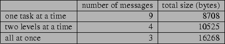
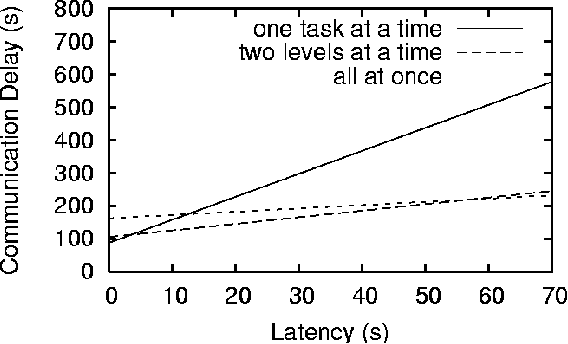 |
| a) |
 |
| b) |
Assuming that the coordinator must wait for requested information
before continuing its search and can request only one task of one
agent at a time, the coordination will be delayed for an amount of
time depending on the bandwidth and latency of message passing. The
total delay can be calculated as ![]() , where
, where ![]() is the
number of messages sent;
is the
number of messages sent; ![]() is the latency in seconds;
is the latency in seconds; ![]() is the
total size of all messages; and
is the
total size of all messages; and ![]() is the bandwidth in bytes per
second. We use
is the bandwidth in bytes per
second. We use ![]() instead of
instead of ![]() because we assume that the agents
all transmit their first top-level summary information message at the
same time, so three messages actually only incur a delay of
because we assume that the agents
all transmit their first top-level summary information message at the
same time, so three messages actually only incur a delay of ![]() instead of
instead of ![]() .
.
Figure 32a shows how the communication delay varies for the three granularities of information for a fixed bandwidth of 100 bytes/second. (We will address the lack of realism in this example shortly.) When the latency is less than 3 seconds, sending summary information for each task in separate messages results in the smallest communication overhead. For latencies greater than 58 seconds, sending the entire hierarchy is best; and in between sending summary information two levels at a time is best. If the latency is fixed at 100 seconds, then the communication delay varies with bandwidth as shown in Figure 32b. When the bandwidth is less than 3 bytes/second, sending one at a time is best; sending it all at once is best for bandwidths greater than 60 bytes/second; and sending two levels at a time is best for bandwidths in between.
Admittedly, these values are unrealistic for the manufacturing domain. The manufacturing problem itself is very simple and provided mainly as an interesting domain for coordination. More realistic problems involving the manufacturing domain could have much larger hierarchies and require much larger scales of data to be sent. In that case more realistic bandwidth and latency values would exhibit similar tradeoffs.
To see this, suppose that the manufacturing managers' hierarchies had
a common branching factor ![]() and depth
and depth ![]() . If tasks generally had
reservations on similar resources throughout the hierarchies, the
amount of total summary information at a particular
level would grow exponentially down the hierarchy just as would the
number of tasks. If the agents agreed on a feasible solution at depth
level
. If tasks generally had
reservations on similar resources throughout the hierarchies, the
amount of total summary information at a particular
level would grow exponentially down the hierarchy just as would the
number of tasks. If the agents agreed on a feasible solution at depth
level ![]() in the hierarchy, then the table for messages and size would
appear as follows:
in the hierarchy, then the table for messages and size would
appear as follows:
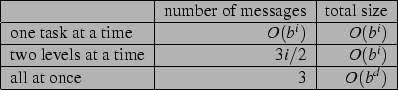
Now suppose that the branching factor ![]() is 3; the depth
is 3; the depth ![]() is 10;
the solution is found at level
is 10;
the solution is found at level ![]() ; and the summary information for
any task is 1 Kbyte. Then the table would look like this:
; and the summary information for
any task is 1 Kbyte. Then the table would look like this:

Now, if we fixed the bandwidth at 100 Kbyte/second and varied the latency, more realistic tradeoffs are seen in Figure 33a. Here, we see that unless the latency is very small, sending summary information two levels at a time is best. As shown in Figure 33b, if we fix latency to be one second and vary the bandwidth, for all realistic bandwidths sending summary information two levels at a time is again best.
This simple protocol illustrates how communication can be minimized by sending summary information at a particular granularity. If the agents chose not to send summary information but the unsummarized hierarchies instead, they would need to send their entire hierarchies. As the experiment shows, as hierarchies grow large, sending the entire hierarchy (``all at once'') would take a long time, even with a high bandwidth. Thus, using summary information (as opposed to not using it) can reduce communication exponentially when solutions can be found at abstract levels.
At the other extreme, if the agents sent summary information one task at a time, the latency for sending so many messages can grow large for larger task hierarchies. If solutions could only be found at primitive levels, then sending summary information one task at a time would cause an exponential latency overhead compared to sending the entire hierarchy at once. But, if solutions can be found at intermediate levels, being able to send summary information at some intermediate granularity can minimize total delay.
However, this argument assumes that summary information collapses at higher levels in the hierarchy. Otherwise, sending summary information at some intermediate level could be almost as expensive as sending the entire hierarchy and cause unnecessary overhead. For the actual manufacturing domain, tasks in the agents' hierarchies mostly have constraints on different resources, and summarization is not able to reduce summary information significantly because constraints do not collapse. The result is that it is better, in this case, to send the entire hierarchy at once to minimize delay (unless there are unusual bandwidth and latency constraints, as shown in the experiment). Even so, the coordination agent can still summarize the hierarchies itself to take advantage of the computational advantages of abstract reasoning.
This section showed how a domain modeler can minimize communication overhead by communicating summary information at the proper level of granularity. If bandwidth, latency, and a common depth for coordination solutions is known, the domain modeler can perform a hypothetical experiment like the one above for varying granularities of summary information to determine which granularity is optimal. If summary information collapses up the hierarchy, and solutions can be found at intermediate levels, then communication can be exponentially reduced in this manner.
The approach we have taken for abstract reasoning was originally inspired by earlier work involving a hierarchical behavior-space search where agents represent their planned behaviors at multiple levels of abstraction [Durfee Montgomery, 1991]. Distributed protocols are used to decide at what level of abstraction coordination is needed and to resolve conflicts there. This approach capitalizes on domains where resources can be abstracted naturally. This earlier work can be viewed as a very limited, special case of the work presented here. It is justified only intuitively and with limited experiments and analyses.
Corkill studied interleaved planning and merging in a distributed version of the NOAH planner corkill:79. He recognized that, while most of the conditions affected by an abstract plan operator might be unknown until further refinement, those that deal with the overall effects and preconditions that hold no matter how the operator is refined can be captured and used to identify and resolve some conflicts. He recognized that further choices of refinement or synchronization choices at more abstract levels could lead to unresolvable conflicts at deeper levels, and backtracking could be necessary. Our work is directed toward avoiding such backtracking by using summary information to guide search.
In closer relation to our approach, Pappachan shows how to interleave hierarchical plan coordination with plan execution for cooperative agents using an online iterative constraint relaxation (OICR) algorithm [Pappachan, 2001]. Like our approach, coordination can be achieved at higher levels of abstraction for more flexible execution, or the agents can decompose their tasks to lower levels for tighter coordination that can improve plan quality. The OICR approach is tailored toward interleaving coordination and flexible execution at the price of completeness while the coordination algorithm presented here is aimed at complete interleaved coordination and planning at the price of potentially delaying execution due to backtracking.
In planning research, hierarchical plans have often been represented as Hierarchical Task Networks (HTNs, erol:94), which planners such as NOAH [Sacerdoti, 1977], NonLin [Tate, 1977], SIPE-2 [Wilkins, 1990], O-Plan [Currie Tate, 1991], UMCP [Erol, Nau, Hendler, 1994b], and SHOP2 [Nau, Au, Ilghami, Kuter, Murdock, Wu, Yaman, 2003] use to search through combinations of alternative courses of action to achieve goals within a particular context. These actions may be partially ordered, giving timing flexibility during execution [Wilkins, 1990, Currie Tate, 1991]. Our CHiP representation extends HTNs to include temporal extent and partial orderings can be expressed as constraints on the starting and ending timepoints of the action.
Yang presented a method (similar to our summarization) for
preprocessing a plan hierarchy in order to be able to detect
unresolvable conflicts at an abstract level so that the planner could
backtrack from inconsistent search spaces [Yang, 1990]. This
corresponds to the use of ![]() in Section
5.2. However, his approach requires that the
decomposition hierarchy be modeled so that each abstract operator have
a unique main subaction that has the same preconditions and
effects as the parent. We avoid this restriction by analyzing the
subplans' conditions and ordering constraints to automatically compute
the parent's summary conditions.
in Section
5.2. However, his approach requires that the
decomposition hierarchy be modeled so that each abstract operator have
a unique main subaction that has the same preconditions and
effects as the parent. We avoid this restriction by analyzing the
subplans' conditions and ordering constraints to automatically compute
the parent's summary conditions.
While our approach has focused on resolving conflicts among agents, cox:03 have used summary information to exploit synergistic interactions. The idea is that using summary information to identify overlapping effects can help agents skip actions whose effects are achieved by others. thang:03 have used summary information in rescheduling during execution. Their representations are actually subsumed by ours, and their work significantly postdates our first reporting of work in this paper [Clement Durfee, 1999].
DSIPE [desJardins Wolvertondes, 1999] is a distributed version of the SIPE-2 [Wilkins, 1990] hierarchical planning system. In the same way agents can use summary information to reduce communication to just those states for which they have common constraints, DSIPE filters conditions communicated among planners using irrelevance reasoning [Wolverton desJardins, 1998].
The DPOCL (Decompositional Partial-Order Causal-Link) planner
[Young, Pollack, Moore, 1994] adds action decomposition to SNLP [Mc, 1991].
Like other HTN planners, preconditions and high level effects can be
added to abstract tasks in order to help the planner resolve conflicts
during decomposition. In addition, causal links can be specified in
decomposition schemas to isolate external preconditions that DPOCL
must satisfy. However, because these conditions and causal links do
not necessarily capture all of the external conditions of abstract
tasks, the planner does not find solutions at abstract levels and
requires that all tasks be completely decomposed. In addition, DPOCL
cannot determine that an abstract plan has unresolvable conflicts
(![]() ) because there may be effects hidden in the
decompositions of yet undetailed tasks that could achieve open
preconditions. By deriving summary conditions automatically and using
algorithms for determining causal link information
(e.g. must-achieve), our planning/coordination algorithm can find and reject abstract plans
during search without adding burden to the domain expert to specify
redundant conditions or causal links for abstract tasks.
) because there may be effects hidden in the
decompositions of yet undetailed tasks that could achieve open
preconditions. By deriving summary conditions automatically and using
algorithms for determining causal link information
(e.g. must-achieve), our planning/coordination algorithm can find and reject abstract plans
during search without adding burden to the domain expert to specify
redundant conditions or causal links for abstract tasks.
Like DPOCL, TÆMS (a framework for Task Analysis, Environment Modeling, and Simulation) allows the domain modeler to specify a wide range of task relationships [Decker, 1995]. This work offers quantitative methods for analyzing and simulating agents as well as their interactions. While only some of these interactions can be represented and discovered using summary conditions, we discover this information through analysis rather than depending on the model developer to predefine the interactions.
Grosz and Kraus's shared plans model of collaboration [Grosz Kraus, 1995] presents a theory for modeling multiagent belief and intention. While the shared plans work is directed toward cooperative agents, it represents action hierarchies and provides mental models at a higher level than represented in this article. However, our use and analysis of summary information complements Grosz's work by providing a way to automatically represent and efficiently reason about the intentions of agents at multiple levels of abstraction. Future work is needed to understand how summary information can be bridged with mental states of agents to exploit the techniques employed in shared plans and other work based on BDI (belief-desire-intention) models of agents [Rao Georgeff, 1995].
An analysis of hierarchical planning [Yang, 1997] explains that, in the case of interacting subgoals, certain structures of the hierarchy that minimize these interactions can reduce worst case planning complexity exponentially. However, the complexity analyses in Section 6 explain how using summary information can achieve exponential performance gains in addition to those achieved by restructuring plan hierarchies according to Yang's analysis by limiting the decomposition of task hierarchies and compressing the information manipulated by a coordinator, planner, or scheduler.
SHOP2 [Nau, Au, Ilghami, Kuter, Murdock, Wu, Yaman, 2003] is an HTN planner that uses a domain translation technique to reason about durative action. This however does not express temporal extent in the same way as the planner given here. Our model differs in that it supports ordering relationships on endpoints as well as conditions and effects during an action's execution. While there may be some domain translation that could achieve the expression of similar constraints and solutions for other systems, ours is the only formal model of such expressions in HTN planning.
SIADEX [Castillo, Fdez-Olivares, García-Pérez, Palao, 2006] is another HTN planner that handles temporal extent in the use of more expressive simple temporal networks [Dechter, Meiri, Pearl, 1991]. The performance improvement techniques reported for SIADEX are in temporal reasoning and not specific to HTNs. Thus, this work is complementary to ours. However, more work is needed to understand how summary information can be exploited in conjunction with the forward expansion approach that both SHOP2 and SIADEX use to perform competitively on planning competition problems.
Another class of hierarchical planners based on ABSTRIPS [Sacerdoti, 1974] introduces conditions at different levels of abstraction so that more critical conflicts are handled at higher levels of abstraction and less important (or easier) conflicts are resolved later at lower levels. While this approach similarly resolves conflicts at abstract levels, the planning decisions may not be consistent with conditions at lower levels resulting in backtracking. Summary information provides a means to make sound and complete decisions at abstract levels without the need to decompose and check consistency with lower levels. However, resolving conflicts based on criticality can still improve performance in complement to our approach.
Allen's temporal planner allen:91 uses hierarchical representations of tasks and could be applied to reasoning about the concurrent actions of multiple agents. However, it does not exploit hierarchy by reasoning about abstraction levels separately and generates a plan by proving the consistency of the collective constraints. Allen's model of temporal plans allen:83b and subsequent work on interval point algebra [Vilain Kautz, 1986] strongly influenced our hierarchical task representation and algorithms that reason about them.
There are also many, many models and theories of concurrency. Some
older examples include automata representations, Petri nets and
Hoare's theory of communicating sequential processes
[Glabbeek, 1997]. There are also many temporal logics such as
computational tree logic (CTL, ctl) that allow modal
expressions about a proposition holding in some or all possible worlds
some of the time, all of the time, in the next state, eventually, or
until some other proposition holds. Another language for specifying
manufacturing processes has been in the process of being standardized
over 10 years [Bock, 1996, Schlenoff, Knutilla, Ray, 2006]. Many of these logics could have been
used to define summary conditions and relations like ![]() .
However, we found that these logics were awkward for representing
inconditions and defining summary conditions and that the terminology
used in this article simplifies the definitions.
.
However, we found that these logics were awkward for representing
inconditions and defining summary conditions and that the terminology
used in this article simplifies the definitions.
Model checking uses temporal logics to verify different properties of system models, software, and hardware (such as correctness, deadlock-free, and convergence). In fact, model checking and planning algorithms can be used interchangeably on the same problems []<e.g.,>giunchiglia:99. In the context of model checking, summary information is a set of properties (akin to those specifiable in CTL) of a system model (as a planning domain) that summarize system variable requirements (conditions) and assignments (effects). Thus, a model checking algorithm could use this summary information to efficiently identify and resolve potential requirement violations/bugs (condition conflicts) or deadlock (resource conflicts) in a system model or its operation (planning/scheduling problem instantiations).
This article provides a formalization of Hierarchical Task Network planning that, unlike the UMCP formalism [Erol, Nau, Hendler, 1994b], includes actions with temporal extent. We introduce a sound and complete algorithm that can be used to generate a plan, coordinate a group of agents with hierarchical plans, and interleave planning and coordination.
The algorithms for summarizing propositional state and metric resource
conditions and effects at abstract levels and the mechanisms that
reason about this summary information can facilitate the construction
of other planning and coordination systems that reason about plans at
multiple levels of abstraction. These mechanisms for reasoning about summary information determine whether a
task (at any level of abstraction) must or may achieve, clobber, or
undo a condition of another task under partial order constraints on
endpoints of tasks. Built on these mechanisms, other mechanisms determine
whether a group of agents can decompose and execute a set of partially
ordered abstract tasks in any way (![]() ), might decompose and
execute them in some way (
), might decompose and
execute them in some way (![]() ), or cannot execute them
consistently in any way (
), or cannot execute them
consistently in any way (![]() ).
).
These algorithms enable a planning system to find solutions at multiple levels of abstraction without needing to fully detail the task hierarchy. These abstract solutions support flexible execution by remaining uncommitted about which of the alternative methods will be selected at runtime, based on the circumstances, to achieve plan subgoals.
Our complexity analyses and experiments in different problem domains
have quantified the benefits of using summary information for a
refinement planning and local search scheduling algorithm. There is a
potential doubly exponential speedup of ![]() for
for ![]() ways to resolve a
conflict, a hierarchy branching factor
ways to resolve a
conflict, a hierarchy branching factor ![]() , a
depth of the hierarchy
, a
depth of the hierarchy ![]() , and an abstract solution depth
, and an abstract solution depth ![]() . An
exponential speedup is obtained if abstract solutions are found, if
there are fewer summary conditions at abstract levels, or if alternative
decomposition choices lead to varying numbers of threats.
These conditions for exponential improvement are a
significant relaxation compared to prior work, and the performance improvement is greater.
. An
exponential speedup is obtained if abstract solutions are found, if
there are fewer summary conditions at abstract levels, or if alternative
decomposition choices lead to varying numbers of threats.
These conditions for exponential improvement are a
significant relaxation compared to prior work, and the performance improvement is greater.
A domain modeler can run the summarization algorithms offline for a library of plan hierarchies so that summary information is available for the coordination and planning of any set of goal tasks supported by the library. Using algorithms for reasoning about summary information, agents can discover with whom they should coordinate and over which states and resources they must coordinate/negotiate. Communicating summary information at different levels of abstraction reduces communication costs exponentially under conditions similar to those reducing computation time.
The use of summary information in a local search planner (like ASPEN, Section 6.3) is another contribution of this work. The strength of local search algorithms is their ability to efficiently reason about large numbers of tasks with constraints on metric resources, state variables, and other complex resource classes. By integrating algorithms for reasoning about summarized propositional state and metric resource constraints into a heuristic local search planner/scheduler, we enable such scalable planning systems to scale to even larger problem domains. This use of summary information in a different style of planner demonstrates the applicability of abstract reasoning in improving the performance of different kinds of planning (and plan coordination) systems.
Future work is needed to evaluate the use of summary information in other planning and scheduling systems and for wider classes of problems requiring more expressive representations for resources and temporal constraints. Already, an approach for exploiting cooperative action among agents based on summary information has been developed [Cox Durfee, 2003]. Other promising approaches include abstracting other plan information, such as probabilistic conditions and effects and classes of resources and states (e.g. location regions and sub-regions). More work is also needed to understand how and when to communicate summary information in a distributed planning system.
The authors wish to thank Pradeep Pappachan, Gregg Rabideau, and Russell Knight for help with implementation. We also thank our anonymous reviewers for their many valuable suggestions. This work was performed at the Jet Propulsion Laboratory, California Institute of Technology, under contract with the National Aeronautics and Space Administration, and at the University of Michigan supported in part by DARPA (F30602-98-2-0142).
The algorithms for determining whether the defined relations hold
between summary conditions for plans in ![]() use a point algebra
constraint table [Vilain Kautz, 1986]. This point algebra
table is constructed for the interval endpoints corresponding to the
executions of the plans in
use a point algebra
constraint table [Vilain Kautz, 1986]. This point algebra
table is constructed for the interval endpoints corresponding to the
executions of the plans in ![]() ; a row and column for both
; a row and column for both ![]() (start endpoint of execution
(start endpoint of execution ![]() of
of ![]() ) and
) and ![]() (finish endpoint) are added for each plan
(finish endpoint) are added for each plan
![]() . Each cell of the table gives a time point constraint of the
row to the column that can be
. Each cell of the table gives a time point constraint of the
row to the column that can be ![]() ,
, ![]() ,
, ![]() ,
, ![]() ,
, ![]() ,
, ![]() ,
,
![]() , or empty.
, or empty. ![]() means that the points are unconstrained. If a cell is empty, then there are no allowed temporal relations, indicating inconsistency.
Table 1 shows a point algebra table for plans
means that the points are unconstrained. If a cell is empty, then there are no allowed temporal relations, indicating inconsistency.
Table 1 shows a point algebra table for plans ![]() and
and
![]() where they are constrained such that
where they are constrained such that ![]() 's execution contains
that of
's execution contains
that of ![]() . Table 2 shows a table where just the start
of
. Table 2 shows a table where just the start
of ![]() is constrained to be earlier than the start of
is constrained to be earlier than the start of ![]() . Both are
transitive closures of these constraint relations. Table
1 can be computed from Table 2 by
constraining
. Both are
transitive closures of these constraint relations. Table
1 can be computed from Table 2 by
constraining ![]() (by putting
(by putting ![]() in the cell of row
in the cell of row
![]() and column
and column ![]() ) and then computing the transitive
closure, an
) and then computing the transitive
closure, an ![]() algorithm for
algorithm for ![]() points [Vilain Kautz, 1986]. After
the transitive closure is computed, the constraints of any point on
any other point can be looked up in constant time.
points [Vilain Kautz, 1986]. After
the transitive closure is computed, the constraints of any point on
any other point can be looked up in constant time.
Similarly, the constraints in ![]() for
for ![]() can be added to the
table, and the transitive closure can be computed to get all
constraints entailed from those in
can be added to the
table, and the transitive closure can be computed to get all
constraints entailed from those in ![]() . This only needs to be
done once for any
. This only needs to be
done once for any ![]() and
and ![]() to determine
to determine ![]() and
and
![]() relationships defined in the next section.
relationships defined in the next section.
We determine that a plan ![]() in
in ![]() 's subplans is temporally ordered
always-[
's subplans is temporally ordered
always-[![]() ,
,![]() ]
if and only if [
]
if and only if [![]() ,
, ![]() ] is
constrained [before, after] or equal to all other points in the point
algebra table for
] is
constrained [before, after] or equal to all other points in the point
algebra table for ![]() 's subplans. This is done by looking at each
entry in the row for [
's subplans. This is done by looking at each
entry in the row for [![]() ,
, ![]() ] and checking to see that the
constraint is [
] and checking to see that the
constraint is [![]() ,
, ![]() ],
], ![]() , or [
, or [![]() ,
, ![]() ]. If this is not
the case, then
]. If this is not
the case, then ![]() is not-always-[
is not-always-[![]() ,
,![]() ].
].
![]() is always-not-[
is always-not-[![]() ,
,![]() ] if and only if in the
row for [
] if and only if in the
row for [![]() ,
, ![]() ] there is an entry with the [
] there is an entry with the [![]() ,
, ![]() ]
constraint; otherwise, it is sometimes-[
]
constraint; otherwise, it is sometimes-[![]() ,
,![]() ].
].
An interval ![]() is covered by a set of intervals
is covered by a set of intervals
![]() if and only no interval can be found that
intersects
if and only no interval can be found that
intersects ![]() and intersects nothing in
and intersects nothing in ![]() . Our particular
covering problem describes the intervals in terms of a partial order
over endpoints, so we represent these intervals in a point algebra
table.
An algorithm for the covering problem is to check to
see if
. Our particular
covering problem describes the intervals in terms of a partial order
over endpoints, so we represent these intervals in a point algebra
table.
An algorithm for the covering problem is to check to
see if ![]() is covered by looking at all pairs of intervals to see if
they overlap.
is covered by looking at all pairs of intervals to see if
they overlap. ![]() is not covered if (1) either no intervals in
is not covered if (1) either no intervals in ![]() meet either
meet either ![]() or
or
![]() , (2) there are any intervals that have an endpoint that is
contained only by
, (2) there are any intervals that have an endpoint that is
contained only by ![]() and do not meet the opposite endpoint of another
interval in
and do not meet the opposite endpoint of another
interval in ![]() or an endpoint of
or an endpoint of ![]() , or (3) there are no intervals
overlapping
, or (3) there are no intervals
overlapping ![]() . Otherwise,
. Otherwise, ![]() is covered. Examples are given in Figure 34.
is covered. Examples are given in Figure 34.
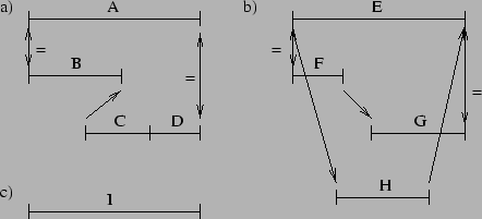 |
Here we describe algorithms for determining temporal plan relationships based on summary information. They are used to build other algorithms that determine whether plan must or may achieve, clobber, or undo the condition of another under particular ordering constraints.
The definitions and algorithms throughout this section are given
within the context of a set of plans ![]() with a corresponding set of
summary information
with a corresponding set of
summary information ![]() , a set of ordering constraints
, a set of ordering constraints ![]() ,
and a set of histories
,
and a set of histories ![]() including all histories where
including all histories where ![]() only
includes an execution
only
includes an execution ![]() of each plan in
of each plan in ![]() and
and ![]() 's subexecutions,
and
's subexecutions,
and ![]() satisfies all constraints in
satisfies all constraints in ![]() . They are all
concerned with the ordering of plan execution intervals and the timing
of conditions. By themselves, they do not have anything to do with
whether conditions may need to be met or must be met for a plan
execution.
. They are all
concerned with the ordering of plan execution intervals and the timing
of conditions. By themselves, they do not have anything to do with
whether conditions may need to be met or must be met for a plan
execution.
First, in order to determine whether abstract plan executions can achieve, clobber, or undo conditions of others, an agent needs to be able to reason about how summary conditions are asserted and required to be met. Ultimately, the agent needs to be able to determine whether a partial ordering of abstract plans can succeed, so it may be the case that an agent's action fails to assert a summary condition that is required by the action of another agent. Therefore, we formalize what it means for an action to attempt to assert a summary condition and to require that a summary condition be met. These definitions rely on linking the summary condition of a plan to the CHiP conditions it summarizes in the subplans of the plan's decompositions. Thus, we first define what it means for a summary condition to summarize these conditions.
A summary conditionsummarizes a condition
in condition set
of plan
iff
;
; and either
, or
For example, ![]() (bin1, A) is a precondition of the
(bin1, A) is a precondition of the ![]() plan
for moving part A from bin1 to machine M1 (as given in Section
2.2). When deriving the summary conditions for
plan
for moving part A from bin1 to machine M1 (as given in Section
2.2). When deriving the summary conditions for ![]() ,
,
![]() (bin1, A) is added to the summary preconditions. Thus, the
summary precondition
(bin1, A) is added to the summary preconditions. Thus, the
summary precondition ![]() (bin1, A)MuF summarizes
(bin1, A)MuF summarizes
![]() (bin1, A) in the preconditions of
(bin1, A) in the preconditions of ![]() .
.
An executionof
iff
,
; if
,
; if
,
; and if
, there is an execution of a subplan of
that requires a summary condition
to be met at
So, basically, an execution requires a summary condition to be met
whenever the conditions it summarizes are required. The execution of ![]() has a summary
precondition
has a summary
precondition ![]() (A,M1_tray1). This execution requires
this summary condition to be met at
(A,M1_tray1). This execution requires
this summary condition to be met at ![]() (
(![]() ) because
) because ![]() (A,
M1_tray1) is a precondition of
(A,
M1_tray1) is a precondition of ![]() 's first subplan that is
summarized by
's first subplan that is
summarized by ![]() 's summary precondition.
's summary precondition.
An execution; if
and before the start or end of any other execution that follows
We say that an execution ``attempts'' to assert a summary condition
because asserting a condition can fail due to a simultaneous assertion
of the negation of the condition. Like the example above for
requiring a summary condition, the executions of ![]() ,
,
![]() , and
, and ![]() all assert summary
postconditions that M1 becomes available at
all assert summary
postconditions that M1 becomes available at ![]() (
(![]() ).
).
In order for agents to determine potential interactions among their
abstract plans (such as clobbering or achieving), they need to reason
about when a summary condition is asserted by one plan in relation to
when it is asserted or required by another. Based on interval or
point algebra constraints over a set of abstract plans, an agent
specifically would need to be able to determine whether a plan would
assert a summary condition before or by the time another
plan requires or asserts a summary condition on the same state variable.
In addition, to reason about clobbering inconditions, an agent would
need to determine if a summary condition would be asserted during the
time a summary incondition ![]() was required (asserted in
was required (asserted in ![]() ).
Agents also need to detect when a summary postcondition would be asserted
at the same time as another summary postcondition
).
Agents also need to detect when a summary postcondition would be asserted
at the same time as another summary postcondition ![]() (asserted
when
(asserted
when ![]() ).
).
We do not consider cases where executions attempt
to assert a summary in- or postcondition at the same time an
incondition is asserted because in these cases, clobber relations are
already detected because executions always require the summary
inconditions that they attempt to assert. For example, if ![]() attempted to assert the incondition
that M1 was unavailable at the same time that
attempted to assert the incondition
that M1 was unavailable at the same time that ![]() attempted to
assert the postcondition that M1 was available, the incondition would be clobbered by
the
postcondition.
attempted to
assert the postcondition that M1 was available, the incondition would be clobbered by
the
postcondition.
In the case that the ordering constraints allow for alternative
synchronizations of the abstract plans, the assertions of summary
conditions may come in different orders. Therefore, we formalize
must-assert and may-assert to determine when these
relationships must or may occur respectively. As mentioned at the
beginning of Section 9, this use of
``must'' and ``may'' is based only on disjunctive orderings and not
on the ![]() of summary conditions in different decompositions.
For the following definitions and algorithms of
must- and may-assert, we assume
of summary conditions in different decompositions.
For the following definitions and algorithms of
must- and may-assert, we assume ![]() and
and ![]() are summary conditions of
plans in
are summary conditions of
plans in ![]() .
.
must-assert
and all
of some
that requires
is the top-level execution of
where
,
].
The must-assert algorithm is described in
Table 3. ![]() must-assert
must-assert ![]() by
by ![]() iff
iff ![]() entails
the relationship given for the row corresponding to the type and timing of the two conditions.
Rows of the table indicate the
timing of both summary conditions and the constraints that
entails
the relationship given for the row corresponding to the type and timing of the two conditions.
Rows of the table indicate the
timing of both summary conditions and the constraints that ![]() must dictate for must-assert to be true. 'T' and 'F' in the table
indicate whether the timing in the column is true or false for the
condition. '?' means that timing doesn't matter for that condition in
this case. For example, row 9 says that for the case where
must dictate for must-assert to be true. 'T' and 'F' in the table
indicate whether the timing in the column is true or false for the
condition. '?' means that timing doesn't matter for that condition in
this case. For example, row 9 says that for the case where ![]() is a
is a
![]() (
(![]() ) postcondition of
) postcondition of ![]() , and
, and ![]() is an
incondition of
is an
incondition of ![]() with any timing,
with any timing, ![]() must require that the end
of
must require that the end
of ![]() be before or at the start of
be before or at the start of ![]() in order for
in order for ![]() to
must-assert
to
must-assert ![]() by the time
by the time ![]() is asserted or required.
is asserted or required.
The definitions and algorithms for the other assert relationships are
similar. Tables 4-6 describe the logic for
the other algorithms. For ![]() relationships, the algorithm
returns true iff none of the corresponding ordering constraints in the
table are imposed by (can be deduced from)
relationships, the algorithm
returns true iff none of the corresponding ordering constraints in the
table are imposed by (can be deduced from) ![]() .
.
We illustrate these relationships for the example in Figure
8. In Figure 8a the agents' plans are
unordered with respect to each other. Part G is produced either on
machine M1 or M2 depending on potential decompositions of the
![]() plan.
plan. ![]() must-assert
must-assert ![]() ,
,
![]()
![]() (G) before
(G) before ![]() ,
, ![]()
![]() (G) in the
summary preconditions of
(G) in the
summary preconditions of ![]() because no matter how the plans are
decomposed (for all executions and all histories of the plans under
the ordering constraints in the figure), the execution of
because no matter how the plans are
decomposed (for all executions and all histories of the plans under
the ordering constraints in the figure), the execution of ![]() attempts to assert
attempts to assert ![]() before the execution of
before the execution of ![]() requires
requires ![]() to be met. The algorithm verifies this by finding that the end of
to be met. The algorithm verifies this by finding that the end of
![]() is ordered before the start of
is ordered before the start of ![]() (row 1 in Table
3). It is also the case that
(row 1 in Table
3). It is also the case that ![]() may-assert
may-assert ![]() ,
, ![]()
![]() (M2) by
(M2) by ![]() ,
, ![]()
![]() (M2) in the summary preconditions of
(M2) in the summary preconditions of
![]() because the two plans are unordered with respect to each
other, and in some history
because the two plans are unordered with respect to each
other, and in some history ![]() can precede
can precede ![]() .
The algorithm finds that this is true since
.
The algorithm finds that this is true since ![]() is not
constrained to start after the start of
is not
constrained to start after the start of ![]() (row 2 in Table
4).
(row 2 in Table
4).
In Figure 8b, ![]() may-assert
may-assert ![]() ,
, ![]()
![]() (transport1) in
(transport1) in ![]() ,
, ![]()
![]() (transport1) in
(transport1) in ![]() 's summary inconditions because in some
history
's summary inconditions because in some
history ![]() attempts to assert
attempts to assert ![]() during the time that
during the time that
![]() is using transport1 to move part A to machine M2.
In addition,
is using transport1 to move part A to machine M2.
In addition, ![]() must-assert
must-assert ![]() ,
, ![]()
![]() (M2) when
(M2) when ![]() ,
, ![]()
![]() (M2) in
(M2) in ![]() 's summary postconditions because
's summary postconditions because
![]() attempts to assert
attempts to assert ![]() at the same time that
at the same time that
![]() requires
requires ![]() to be met. The end of Section 3.3 gives other examples.
to be met. The end of Section 3.3 gives other examples.
This document was generated using the LaTeX2HTML translator Version 2002-2-1 (1.70)
Copyright © 1993, 1994, 1995, 1996,
Nikos Drakos,
Computer Based Learning Unit, University of Leeds.
Copyright © 1997, 1998, 1999,
Ross Moore,
Mathematics Department, Macquarie University, Sydney.
The command line arguments were:
latex2html -html_version 3.0 -split 0 -toc_depth 4 -show_section_numbers -link 2 -long_titles 3 -white -dir jair06efinal_1_page jair06efinal.tex
The translation was initiated by Bradley Clement on 2006-12-29

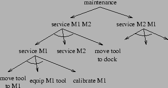

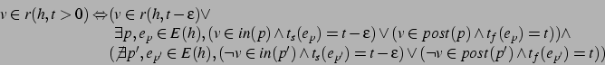

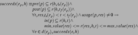

![\begin{displaymath}
\begin{array}{@{}l@{}l@{}l}
[ach&ieves,clobbers]
\_precondit...
...{p''},\neg\ell,t'',h)) \wedge t<t''\leq t_s(e_{p'})
\end{array}\end{displaymath}](img117.png)
![\begin{displaymath}
\begin{array}{@{}l@{}l@{}l}
clob&bers\_[in,post]condition(e_...
...] \wedge [t_s(e_{p'})<t<t_s(e_{p'}), t=t_f(e_{p'})]
\end{array}\end{displaymath}](img118.png)


![\begin{displaymath}
\begin{array}{@{}l@{}l@{}l}
exte&rnal\_[pre,post]condition(\...
...st]condition(e_{p''}, \ell, e_{p'},t,h))
\end{array}\end{array}\end{displaymath}](img122.png)
![\begin{displaymath}
\begin{array}{@{}l@{}l@{}l}
[mu&st,may]\_first\_precondition...
...}) \wedge \ell \in pre(p'')
\end{array} \end{array}\end{array}\end{displaymath}](img165.png)

![\begin{displaymath}
\begin{array}{@{}l@{}l@{}l}
[mus&t,may]\_sometimes\_incondit...
... \ell\in post(p'')
\end{array}\end{array}\end{array}\end{array}\end{displaymath}](img167.png)

![\begin{displaymath}
\begin{array}{@{}l@{}l@{}l}
must&\_[achieve,clobber]
\_preco...
...ndition(\ell(c_2),e_{p_2'})
\end{array} \end{array}\end{array}\end{displaymath}](img184.png)


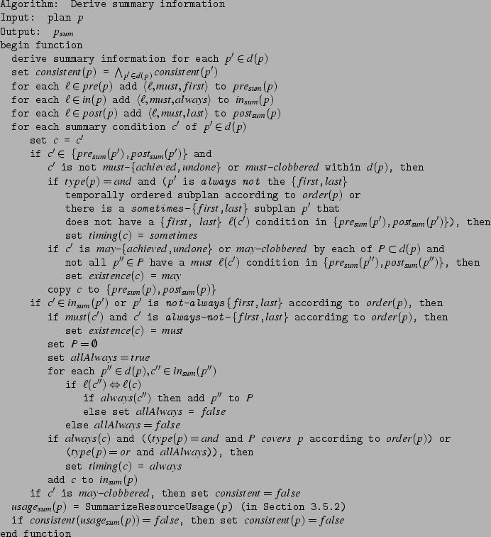

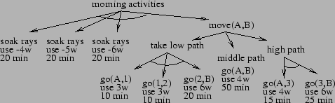
![\begin{displaymath}
\setlength{\arraycolsep}{0in}
\begin{array}[t]{lll}
usage_{...
...p\in E(h)}(-r(res,h,t_f(e_p)))]& \rangle
\end{array}\end{array}\end{displaymath}](img210.png)

, succeeds(e,h)
\end{array}\end{displaymath}](img253.png)