Next: Semantics of HAs Up: Semantics Previous: Semantics of PDDL+
The following definition uses the interpretation of preconditions defined in Core Definition 9. This core definition explains how, given a proposition ![]() and a logical state
and a logical state ![]() , the truth of the proposition is determined.
, the truth of the proposition is determined. ![]() is a predicate over the PNEs in the domain. As explained in Core Definition 9, to determine the truth of a proposition in a state, with respect to a vector of numeric values
is a predicate over the PNEs in the domain. As explained in Core Definition 9, to determine the truth of a proposition in a state, with respect to a vector of numeric values ![]() , the formal numeric parameters of the proposition are substituted with the values in
, the formal numeric parameters of the proposition are substituted with the values in ![]() and the resulting proposition is evaluated in the logical state. The purpose of Definition 7 is to identify actions, events or processes that could be applicable in a given logical state, if the values of the metric fluents are appropriate to satisfy their preconditions.
and the resulting proposition is evaluated in the logical state. The purpose of Definition 7 is to identify actions, events or processes that could be applicable in a given logical state, if the values of the metric fluents are appropriate to satisfy their preconditions.
![]() (
(
![]() ) is the set of all ground processes (events) that are relevant in state
) is the set of all ground processes (events) that are relevant in state ![]() .
.
In the construction of a HA, in the mappings described below, the vertices of its control graph are subsets of ground atoms and are therefore equivalent to logical states. We use the variable ![]() to denote a vertex and
to denote a vertex and
![]() (
(
![]() ) to denote the processes (events) relevant in the corresponding logical state.
) to denote the processes (events) relevant in the corresponding logical state.
In any given logical state a subset of the relevant processes will be active, according to the precise valuation of the metric fluents in the current state. We first consider the restricted case in which no more than one active process affects the value of each variable at any time, which we call a uniprocess planning instance. The proposition unary-context-flow(![]() ,
,![]() ), defined below, is used to describe the effects on the
), defined below, is used to describe the effects on the ![]() th variable of the process
th variable of the process ![]() , when it is active. We later extend this definition to the concurrent case in which multiple processes may contribute to the behaviour of a variable.
, when it is active. We later extend this definition to the concurrent case in which multiple processes may contribute to the behaviour of a variable.
We begin by presenting the semantics of a event-free uniprocess planning instance -- that is, a uniprocess planning instance that contains no events. We then extend our definition to include events, and present the semantics of a uniprocess planning instance. Finally we introduce concurrent process effects and the definition of the semantics of a planning instance.
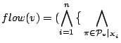
The vertex labelling function flow is defined:
To illustrate this construction we now present a simple example. The planetary lander domain requires events and so cannot be used as an example of the event-free model. Consider the PDDL+ domain containing just the following actions and process:
(:action startEngine
 :precondition (stopped)
 :effect (and (not (stopped))
              (running))
)

(:action accelerate
 :precondition (running)
 :effect (increase (a) 1)
)

(:action decelerate
 :precondition (running)
 :effect (decrease (a) 1)
)

(:action stop
 :precondition (and (= (v) 0) (running))
 :effect (and (not (running))
              (stopped)
              (assign (a) 0))
)

(:process moving
 :precondition (running)
 :effect (and (increase (d) (* #t (v)))
              (increase (v) (* #t (a))))
)
The translation process described in Definition 10 leads to the hybrid automaton shown in Figure 10. As can be seen, there are two vertices, corresponding to the logical states
![\includegraphics[width=10cm]{haeg1}](img123.png) |
We now consider the case in which events are included but there can only be one process active on any one fluent at any one time.
In planning domains it is important to distinguish between state changes that are deliberately planned, called actions, and those, called events, that are brought about spontaneously in the world. There is no such distinction in the HA, where all control switches are called events. This distinction complicates the relationship between plans and traces, because plans contain only the control switches that correspond to actions. Any events triggered by the evolution of the domain under the influence of planned actions must be inferred and added to the sequence of actions in order to arrive at the corresponding traces.
Henzinger et al. henzingerdecides discuss the use of ![]() -moves, which are transitions that are not labelled with a corresponding control-switch, but with the special label
-moves, which are transitions that are not labelled with a corresponding control-switch, but with the special label ![]() . The significance of these transitions is that they do not appear in traces. A trace that corresponds to an accepting run using
. The significance of these transitions is that they do not appear in traces. A trace that corresponds to an accepting run using ![]() -moves will contain only those transitions that are labelled with elements from
-moves will contain only those transitions that are labelled with elements from ![]() . Where
. Where ![]() -moves appear between time transitions, the lengths of these transitions can be accumulated into a single transition in the corresponding trace. The purpose of these silent transitions is that they allow special book-keeping transitions to be inserted into automata that can be used to simulate automata with syntactically richer constraints, allowing various reducibility results to be demonstrated. The convenient aspect of the
-moves appear between time transitions, the lengths of these transitions can be accumulated into a single transition in the corresponding trace. The purpose of these silent transitions is that they allow special book-keeping transitions to be inserted into automata that can be used to simulate automata with syntactically richer constraints, allowing various reducibility results to be demonstrated. The convenient aspect of the ![]() -moves is that they do not affect traces when they are transferred from the original automata to the simulations.
-moves is that they do not affect traces when they are transferred from the original automata to the simulations.
In PDDL+, events are similar to ![]() -moves in that they do not appear explicitly in plans. However, in contrast to
-moves in that they do not appear explicitly in plans. However, in contrast to ![]() -moves, applicable events are always forced to occur before any actions may be applied in a state.
-moves, applicable events are always forced to occur before any actions may be applied in a state.
When extending event-free planning instances to include events we require a mechanism for capturing the fact that events occur at the instant at which they are triggered by the world, and not at the convenience of the planner. No time must be allowed to pass between the satisfaction of event preconditions and the triggering of the event. In our semantic models we use a variable to measure the amount of time that elapses between the preconditions of an event becoming true and the event triggering. Obviously this quantity, which we call time-slip, must be 0 in any valid planning instance. In the HA that we construct we associate an invariant with each vertex in the control graph to enforce this requirement. It might appear that a simpler way to handle events would be to simply assert that an invariant condition for each state is that the preconditions of all events are false, while each event is represented by an outgoing transition with a jump condition specifying the precondition of the corresponding event. However, it is not possible for a jump condition on a transition to be inconsistent with the invariant of the state it leaves since both must hold simultaneously at the time at which the transition is made.
The variable used to monitor time-slip for a planning instance of dimension ![]() is the variable
is the variable ![]() . This variable operates as a clock tracking the passage of time once an event becomes applicable. We define the time-slippage proposition to switch the clock on whenever the preconditions of any event become true in any state. When no event is applicable the clock is switched off.
. This variable operates as a clock tracking the passage of time once an event becomes applicable. We define the time-slippage proposition to switch the clock on whenever the preconditions of any event become true in any state. When no event is applicable the clock is switched off.

The interpretation of a Uniprocess Planning Instance extends the interpretation of the Event-free Uniprocess Planning Instance. The added components are underlined for ease of comparison.
The vertex labelling function flow is defined:
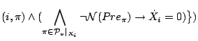
Given an edge ![]() from vertex
from vertex ![]() , associated with an event
, associated with an event ![]() :
:
(:event engineExplode
 :parameters ()
 :precondition (and (running) (>= (a) 1) (>= (v) 100))
 :effect (and (not (running)) (assign (a) 0) (engineBlown))
)
The corresponding machine is shown in Figure 11. The structure of this machine is similar to the previous example, but includes an extra state, reachable by an event transition. The addition of an event also requires the addition of the time-slip variable, ![]() . The behaviour of this variable is controlled, in particular, by a new flow constraint in the running state that ensures that if the event precondition becomes true then the time-slip starts to increase as soon as any time passes. The addition of this variable and its control also propagates into the jump and flow conditions of the other states.
. The behaviour of this variable is controlled, in particular, by a new flow constraint in the running state that ensures that if the event precondition becomes true then the time-slip starts to increase as soon as any time passes. The addition of this variable and its control also propagates into the jump and flow conditions of the other states.
Finally we consider the case in which concurrent process effects occur and must be combined. This is the general case to which we refer in the rest of this paper.
In any given logical state a subset of the relevant processes will be active, according to the precise valuation of the metric fluents in the current state. The proposition context-flow(i,![]() ) asserts that the rate of change of the
) asserts that the rate of change of the ![]() th variable is defined by precisely those processes in
th variable is defined by precisely those processes in ![]() , provided that they (and only they) are all active, and is not affected by any other process. The following definition explains how the contributions to the rate of change of a variable by several different concurrent processes are combined (see also Section 4.2). This simply involves summing the contributions that are active at an instant. Here we assume without loss of generality that contributions are increasing effects. Decreasing effects are handled by simply negating the contributions made by these effects.
, provided that they (and only they) are all active, and is not affected by any other process. The following definition explains how the contributions to the rate of change of a variable by several different concurrent processes are combined (see also Section 4.2). This simply involves summing the contributions that are active at an instant. Here we assume without loss of generality that contributions are increasing effects. Decreasing effects are handled by simply negating the contributions made by these effects.
It will be noted that if ![]() contains no processes that affect a specific variable,
contains no processes that affect a specific variable, ![]() , then
, then
![]() .
.
If ![]() is empty then the context flow proposition asserts that
is empty then the context flow proposition asserts that
![]() for each
for each ![]() .
.
The interpretation of a Planning Instance extends the interpretation of a Uniprocess Planning Instance. Again, the added components are underlined for convenience.
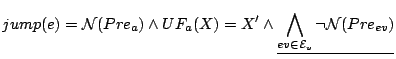
The vertex labelling function flow is defined:

Given an edge ![]() from vertex
from vertex ![]() , associated with an event
, associated with an event ![]() :
:
The final conjunct in the jump definition for actions ensures that the state cannot be left by an action if there is an event the preconditions of which are satisfied. It is possible for more than one event to be simultaneously applicable in the same state. This is discussed further in Section 6.4.
As an illustration of this final extension in the sequence of definitions, we now add one further process to the preceding example:
(:process windResistance
 :parameters ()
 :precondition (and (running) (>= (v) 50))
 :effect (decrease (v) (* #t (* 0.1 (* (- (v) 50) (- (v) 50)))))
)
This process causes the vehicle to be slowed by a wind resistance that becomes effective from 50mph, and is proportional to the square of the speed excess over 50mph. This leads to the flow constraint in the running state having two new clauses that replace the original constraint on the rate of change of velocity. These new clauses are shown in the second box out on the right of Figure 12. As can be observed, the velocity of the vehicle is now governed by two different differential equations, according to whether ![]() or
or ![]() . These equations are:
. These equations are:
The definition of the semantics of a planning instance is constructed around a basic framework of the discrete state space model of the domain. This follows a familiar discrete planning model semantics. The continuous dimensions of the model are constructed to ensure that the Hybrid Automaton will always start in an initial state consistent with the planning instance (modelled by the init labelling function). The state invariants ensure that no time-slip occurs in the model and that, therefore, events always occur once their preconditions are satisfied. It will be noted that since the negation of the event preconditions is added to all jump conditions for other exiting transitions, it will be impossible for a state to be exited in any other way than by the triggered event. Finally, flow models the effect on the real values of all of the active processes in a state. The flow function assigns a proposition to each state that determines a piece-wise continuous behaviour for each of the real values in the planning domain. The function is piece-wise differentiable, with only a finite number of segments within any finite interval. The reason for this is that it is possible for the behaviour of a metric fluent undergoing continuous change to affect the precondition of a process and cause the continuous change in itself or of other metric fluents to change. Such a change cannot cause discontinuity in the value of the metric fluents themselves, but it can cause discontinuity in the derivatives. The consequence of this is that the time interval between two successive actions or events might include a finite sequence of distinct periods of continuous change. As will be seen in the following section, this requires that an acceptable trace describing such behaviour will explicitly subdivide the interval into a sequence of subintervals in each of which the continuous change is governed by a stable set of differential equations.
Derek Long 2006-10-09
![\includegraphics[width=13cm]{haeg3}](img139.png)
![\includegraphics[width=13cm]{haeg4}](img168.png)