Heuristics

This section discusses how we can use planning graph heuristics to measure belief state distances. We cover several types of planning graphs and the extent to which they can be used to compute various heuristics. We begin with a brief background on planning graphs.

Planning Graphs: Planning graphs serve as the basis for our belief state distance estimation. Planning graphs were initially introduced in GraphPlan [4] for representing an optimistic, compressed version of the state space progression tree. The compression lies in unioning the literals from every state at subsequent steps from the initial state. The optimism relates to underestimating the number of steps it takes to support sets of literals (by tracking only a subset of the infeasible tuples of literals). GraphPlan searches the compressed progression (or planning graph) once it achieves the goal literals in a level with no two goal literals marked infeasible. The search tries to find actions to support the top level goal literals, then find actions to support the chosen actions and so on until reaching the first graph level. The basic idea behind using planning graphs for search heuristics is that we can find the first level of a planning graph where a literal in a state appears; the index of this level is a lower bound on the number of actions that are needed to achieve a state with the literal. There are also techniques for estimating the number of actions required to achieve sets of literals. The planning graphs serve as a way to estimate the reachability of state literals and discriminate between the ``goodness'' of different search states. This work generalizes such literal estimations to belief space search by considering both GraphPlan and CGP style planning graphs plus a new generalization of planning graphs, called the $LUG$ .

Planners such as CGP [30] and SGP [31] adapt the GraphPlan idea of compressing the search space with a planning graph by using multiple planning graphs, one for each possible world in the initial belief state. CGP and SGP search on these planning graphs, similar to GraphPlan, to find conformant and conditional plans. The work in this paper seeks to apply the idea of extracting search heuristics from planning graphs, previously used in state space search [23,18,5] to belief space search.

Planning Graphs for Belief Space: This section proceeds by describing four classes of heuristics to estimate belief state distance $NG, SG, MG,$ and $LUG$ . $NG$ heuristics are techniques existing in the literature that are not based on planning graphs, $SG$ heuristics are techniques based on a single classical planning graph, $MG$ heuristics are techniques based on multiple planning graphs (similar to those used in CGP) and $LUG$ heuristics use a new labelled planning graph. The $LUG$ combines the advantages of $SG$ and $MG$ to reduce the representation size and maintain informedness. Note that we do not include observations in any of the planning graph structures as SGP [31] would, however we do include this feature for future work. The conditional planning formulation directly uses the planning graph heuristics by ignoring observations, and our results show that this still gives good performance.

Figure 4: Taxonomy of heuristics with respect to planning graph type and state distance aggregation. Blank entries indicate that the combination is meaningless or not possible.

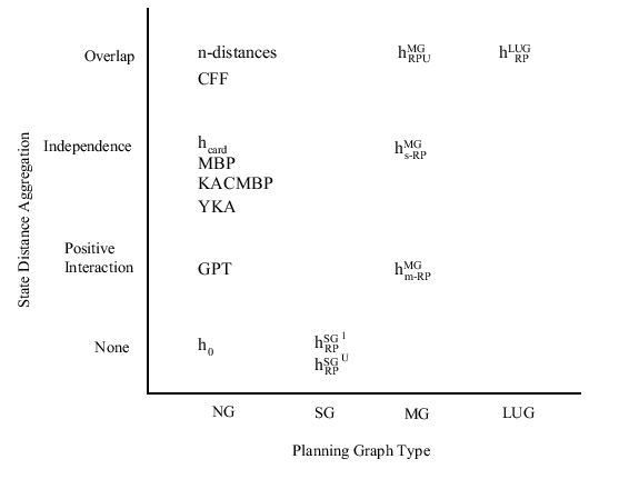
In Figure 4 we present a taxonomy of distance measures for belief space. The taxonomy also includes related planners, whose distance measures will be characterized in this section. All of the related planners are listed in the $NG$ group, despite the fact that some actually use planning graphs, because they do not clearly fall into one of our planning graph categories. The figure shows how different substrates (horizontal axis) can be used to compute belief state distance by aggregating state to state distances under various assumptions (vertical axis). Some of the combinations are not considered because they do not make sense or are impossible. The reasons for these omissions will be discussed in subsequent sections. While there are a wealth of different heuristics one can compute using planning graphs, we concentrate on relaxed plans because they have proven to be the most effective in classical planning and in our previous studies [9]. We provide additional descriptions of other heuristics like max, sum, and level in Appendix A.

Example: To illustrate the computation of each heuristic, we use an example derived from BTC called Courteous BTC (CBTC) where a courteous package dunker has to disarm the bomb and leave the toilet unclogged, but some discourteous person has left the toilet clogged. The initial belief state of CBTC in clausal representation is:

$\kappa(BS_I) =$ arm $\wedge$ clog $\wedge$ (inP1 $\vee$ inP2) $\wedge$ ($\neg$ inP1 $\vee \neg$ inP2),

and the goal is:

$\kappa(BS_G) =$ $\neg$ clog $\wedge \neg$ arm.

The optimal action sequences to reach $BS_G$ from $BS_I$ are:

Flush, DunkP1, Flush, DunkP2, Flush,

and

Flush, DunkP2, Flush, DunkP1, Flush.

Thus the optimal heuristic estimate for the distance between $BS_I$ and $BS_G$ , in regression, is $h^{*}(BS_G)$ = 5 because in either plan there are five actions.

We use planning graphs for both progression and regression search. In regression search the heuristic estimates the cost of the current belief state w.r.t. the initial belief state and in progression search the heuristic estimates the cost of the goal belief state w.r.t. the current belief state. Thus, in regression search the planning graph(s) are built (projected) once from the possible worlds of the initial belief state, but in progression search they need to be built at each search node. We introduce a notation $BS_i$ to denote the belief state for which we find a heuristic measure, and $BS_P$ to denote the belief state that is used to construct the initial layer of the planning graph(s). In the following subsections we describe computing heuristics for regression, but they are generalized for progression by changing $BS_i$ and $BS_P$ appropriately.

In the previous section we discussed two important issues involved in heuristic computation: sampling states to include in the computation and using mutexes to capture negative interactions in the heuristics. We will not directly address these issues in this section, deferring them to discussion in the respective empirical evaluation sections, 6.4 and 6.2. The heuristics below are computed once we have decided on a set of states to use, whether by sampling or not. Also, as previously mentioned, we only consider sampling states from the belief state $BS_P$ because we can implicitly find closest states from $BS_i$ without sampling. We only explore computing mutexes on the planning graphs in regression search. We use mutexes to determine the first level of the planning graph where the goal belief state is reachable (via the level heuristic described in Appendix A) and then extract a relaxed plan starting at that level. If the level heuristic is $\infty$ because there is no level where a belief state is reachable, then we can prune the regressed belief state.

We proceed by describing the various substrates used for computing belief space distance estimates. Within each we describe the prospects for various types of world aggregation. In addition to our heuristics, we mention related work in the relevant areas.