Probability and Reward Structure

An action a ∈ A consists of a precondition φ_a and an effect e_a. Action a is applicable in a state s if and only if s $\models$ ¬φ_G∧φ_a. It is an error to apply a to a state such that s $\not\models$ ¬φ_G∧φ_a. Goal states are absorbing, so no action may be applied to a state satisfying φ_G. The requirement that φ_a must hold in order for a to be applicable is consistent with the semantics of PDDL2.1 (Fox & Long, 2003) and permits the modeling of forced chains of actions. Effects are recursively defined as follows (see also, Rintanen, 2003):

1. $\top$ is the null-effect, represented in PPDDL by (and).
2. b and ¬b are effects if b ∈ V is a Boolean state variable.
3. r ↑ v, for v ∈ $\mathbb {R}$, is an effect.
4. c$\vartriangleright$e is an effect if c is a formula over V and e is an effect.
5. e₁∧ ^... ∧e_n is an effect if e₁,..., e_n are effects.
6. p₁e₁|...| p_ne_n is an effect if e₁,..., e_n are effects, p_i ≥ 0 for all i ∈ {1,..., n}, and $\sum_{{i=1}}^{n}$p_i = 1.

The effect b sets the Boolean state variable b to true in the next state, while ¬b sets b to false in the next state. Effects of the form r ↑ v are used to associate rewards with transitions as described below.

An action a = $\langle$φ_a, e_a$\rangle$ defines a transition probability matrix P_a and a state reward vector R_a, with P_a(i, j) being the probability of transitioning to state j when applying a in state i, and R_a(i) being the expected reward for executing action a in state i. We can readily compute the entries of the reward vector from the action effect formula e_a. Let χ_c be the characteristic function for the Boolean formula c, that is, χ_c(s) is 1 if s $\models$ c and 0 otherwise. The expected reward for an effect e applied to a state s, denoted R(e;s), can be computed using the following inductive definition:

R($$\top$$;s)	=	0
R(b;s)	=	0
R(¬b;s)	=	0
R(r ↑ v;s)	=	v
R(c$$\vartriangleright$$e;s)	=	χc(s) . R(e;s)
R(e1∧ ... ∧en;s)	=	$\sum_{{i=1}}^{n}$R(ei; s)
R(p1e1|...| pnen;s)	=	$\sum_{{i=1}}^{n}$pi . R(ei; s)

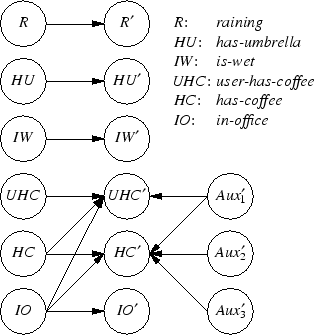
A factored representation of the probability matrix P_a can be obtained by generating a dynamic Bayesian network (DBN) representation of the action effect formula e_a. We can use Bayesian inference on the DBN to obtain a monolithic representation of P_a, but the structure of the factored representation can be exploited by algorithms for decision theoretic planning (see, for example, work by Boutilier, Dearden, & Goldszmidt, 1995,Hoey, St-Aubin, Hu, & Boutilier, 1999,Boutilier, Dean, & Hanks, 1999,Guestrin, Koller, Parr, & Venkataraman, 2003).

A Bayesian network is a directed graph. Each node of the graph represents a state variable, and a directed edge from one node to another represents a causal dependence. With each node is associated a conditional probability table (CPT). The CPT for state variable X's node represents the probability distribution over possible values for X conditioned on the values of state variables whose nodes are parents of X's node. A Bayesian network is a factored representation of the joint probability distribution over the variables represented in the network.

A DBN is a Bayesian network with a specific structure aimed at capturing temporal dependence. For each state variable X, we create a duplicate state variable X′, with X representing the situation at the present time and X′ representing the situation one time step into the future. A directed edge from a present-time state variable X to a future-time state variable Y′ encodes a temporal dependence. There are no edges between two present-time state variables, or from a future-time to a present-time state variable (the present does not depend on the future). We can, however, have an edge between two future-time state variables. Such edges, called synchronic edges, are used to represent correlated effects. A DBN is a factored representation of the joint probability distribution over present-time and future-time state variables, which is also the transition probability matrix for a discrete-time Markov process.

We now show how to generate a DBN representing the transition probability matrix for a PPDDL action. To avoid representational blowup, we introduce a multi-valued auxiliary variable for each probabilistic effect of an action effect. These auxiliary variables are introduced to indicate which of the possible outcomes of a probabilistic effect occurs, allowing the representation to correlate all the effects of a specific outcome. The auxiliary variable associated with a probabilistic effect with n outcomes can take on n different values. A PPDDL effect e of size | e| can consist of at most O(| e|) distinct probabilistic effects. Hence, the number of auxiliary variables required to encode the transition probability matrix for an action with effect e will be at most O(| e|). Only future-time versions of the auxiliary variables are necessary. For a PPDDL problem with m Boolean state variables, we need on the order of 2m + $\max_{{a\in A}}^{}$| e_a| nodes in the DBNs representing transition probability matrices for actions.

We provide a compositional approach for generating a DBN that represents the transition probability matrix for a PPDDL action with precondition φ_a and effect e_a. We assume that the effect is consistent, that is, that b and ¬b do not occur in the same outcome with overlapping conditions. The DBN for an empty effect $\top$ simply consists of 2m nodes, with each present-time node X connected to its future-time counterpart X′. The CPT for X′ has the non-zero entries Pr[X′ = $\top$  |  X = $\top$] = 1 and Pr[X′ = ⊥  |  X = ⊥] = 1. The same holds for a reward effect r ↑ v, which does not change the value of state variables.

Next, consider the simple effects b and ¬b. Let X_b be the state variable associated with the PPDDL atom b. For these effects, we eliminate the edge from X_b to X′_b. The CPT for X′_b has the entry Pr[X′_b = $\top$] = 1 for effect b and Pr[X′_b = ⊥] = 1 for effect ¬b.

For conditional effects, c$\vartriangleright$e, we take the DBN for e and add edges between the present-time state variables mentioned in the formula c and the future-time state variables in the DBN for e.¹Entries in the CPT for a state variable X′ that correspond to settings of the present-time state variables that satisfy c remain unchanged. The other entries are set to 1 if X is true and 0 otherwise (the value of X does not change if the effect condition is not satisfied).

The DBN for an effect conjunction e₁∧ ^... ∧e_n is constructed from the DBNs for the n effect conjuncts. The value for Pr[X′ = $\top$  |  X] in the DBN for the conjunction is set to the maximum of Pr[X′ = $\top$  |  X] over the DBNs for the conjuncts. The maximum is used because a state variable is set to true (false) by the conjunctive effect if it is set to true (false) by one of the effect conjuncts (effects are assumed to be consistent, so that the result of taking the maximum over the separate probability tables is still a probability table).

Finally, to construct a DBN for a probabilistic effect p₁e₁|...| p_ne_n, we introduce an auxiliary variable Y′ that is used to indicate which one of the n outcomes occurred. The node for Y′ does not have any parents, and the entries of the CPT are Pr[Y′ = i] = p_i. Given a DBN for e_i, we add a synchronic edge from Y′ to all state variables X. The value of Pr[X′ = $\top$  |  X, Y′ = j] is set to Pr[X′ = $\top$  |  X] if j = i and 0 otherwise. This transformation is repeated for all n outcomes, which results in n DBNs. These DBNs can trivially be combined into a single DBN for the probabilistic effect because they have mutually exclusive preconditions (the value of Y).

As an example, Figure 3 shows the DBN encoding of the transition probability matrix for the “deliver-coffee” action, whose PPDDL encoding was given in Figure 2. There are three auxiliary variables because the action effect contains three probabilistic effects. The node labeled UHC′ (the future-time version of the state variable user-has-coffee) has four parents, including one auxiliary variable. Consequently, the CPT for this node will have 2⁴ = 16 rows (shown to the right in Figure 3).

Figure 3: DBN structure (left) for the “deliver-coffee” action of the “Coffee Delivery” domain, with the CPT for UHC′ (the future-time version of the state variable user-has-coffee) shown to the right.

				UHC′
Aux′1	IO	HC	UHC	$\top$	⊥
1	$\top$	$\top$	$\top$	1	0
1	$\top$	$\top$	⊥	1	0
1	$\top$	⊥	$\top$	1	0
1	$\top$	⊥	⊥	0	1
1	⊥	$\top$	$\top$	1	0
1	⊥	$\top$	⊥	0	1
1	⊥	⊥	$\top$	1	0
1	⊥	⊥	⊥	0	1
2	$\top$	$\top$	$\top$	1	0
2	$\top$	$\top$	⊥	0	1
2	$\top$	⊥	$\top$	1	0
2	$\top$	⊥	⊥	0	1
2	⊥	$\top$	$\top$	1	0
2	⊥	$\top$	⊥	0	1
2	⊥	⊥	$\top$	1	0
2	⊥	⊥	⊥	0	1