Estimation of the Weights of the Networks of an Ensemble

Neural network ensembles [PC93] [GPHMOB05] are receiving increasing attention in recent neural network research, due to their interesting features. They are a powerful tool specially when facing complex problems. Network ensembles are made up of a linear combination of several networks that have been trained using the same data, although the actual sample used by each network to learn can be different. Each network within the ensemble has a potentially different weight in the output of the ensemble. Several papers have shown [PC93] that the network ensemble has a generalization error generally smaller than that obtained with a single network and also that the variance of the ensemble is lesser than the variance of a single network. The output of an ensemble, $y$, when an input pattern $\mathbf x$ is presented, is:

$$y({\mathbf x}) = \sum_{i=1}^k \alpha_i y_i ({\mathbf x}),$$ (15)

where $y_i$ is the output of network $i$, and $w_i$ is the weight associated to that network. If the networks have more than one output, a different weight is usually assigned to each output. The ensembles of neural networks have some of the advantages of large networks without their problems of long training time and risk of over-fitting.

Moreover, this combination of several networks that cooperate in solving a given task has other important advantages, such as [LYH00,Sha96]:

• They can perform more complex tasks than any of their subcomponents.
• They can make an overall system easier to understand and modify.
• They are more robust than a single network.

Techniques using multiple models usually consist of two independent phases: model generation and model combination [Mer99b]. Once each network has been trained and assigned a weights (model generation), there are, in a classification environment three basic methods for combining the outputs of the networks (model combination):

1. Majority voting. Each pattern is classified into the class where the majority of networks places it [Mer99b]. Majority voting is effective, but is prone to fail in two scenarios:
   1. When a subset of redundant and less accurate models comprise the majority, and
   2. When a dissenting vote is not recognized as an area of specialization for a particular model.

2. Sum of the outputs of the networks. The output of the ensemble is just the sum of the outputs of the individual networks.

3. Winner takes all. The pattern is assigned to the class with the highest output over all the outputs of all the networks. That is, the network with the largest outputs directly classify the pattern, without taking into account the other networks.

The most commonly used methods for combining the networks are the majority voting and sum of the outputs of the networks, both with a weight vector that measures the confidence in the prediction of each network. The problem of obtaining the weight vector $\boldsymbol{\alpha}$ is not an easy task. Usually, the values of the weights $\alpha_i$ are constrained:

$$\sum_{i=1}^N \alpha_i = 1,$$ (16)

in order to help to produce estimators with lower prediction error [LT93], although the justification of this constraint is just intuitive [Bre96]. When the method of majority voting is applied, the vote of each network is weighted before it is counted:

$$F(\boldsymbol{x}) = _{y} \sum_{i:f_i(\boldsymbol{x})=y} \alpha_i.$$ (17)

The problem of finding the optimal weight vector is a very complex task. The ``Basic ensemble method (BEM)'', as it is called by Perrone and Cooper [PC93], consists of weighting all the networks equally. So, having $N$ networks, the output of the ensembles is:

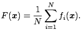$$F(\boldsymbol{x}) = {1 \over N} \sum_{i=1}^N f_i(\boldsymbol{x}).$$ (18)

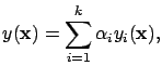
Perrone and Cooper [PC93] defined the Generalized Ensemble Method, which is equivalent to the Mean Square Error - Optimal Linear Combination (MSE-OLC) without a constant term of Hashem [Has97]. The form of the output of the ensemble is:

$$f_{GEM}(\boldsymbol{x}) \equiv \sum_{i=1}^N \alpha_i f_i(\boldsymbol{x}),$$ (19)

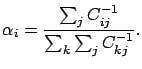
where the $\alpha_i's$ are real and satisfy the constraint $\sum_{i=1}^N \alpha_i = 1$. The values of $\alpha_i$ are given by:

$$\alpha_i = {\sum_j C_{ij}^{-1} \over \sum_k \sum_j C_{kj}^{-1}}.$$ (20)

where $C_{ij}$ is the symmetric correlation matrix $C_{ij} \equiv E[m_i(\boldsymbol{x})m_j(\boldsymbol{x})]$, where $m_k(\boldsymbol{x})$ defines the misfit of function $k$, that is the deviation from the true solution $f(\boldsymbol{x})$, $m_k(\boldsymbol{x}) \equiv f(\boldsymbol{x}) - f_k(\boldsymbol{x})$. The previous methods are commonly used. Nevertheless, many other techniques have been proposed over the last few years. Among others, there are methods based on linear regression [LT93], principal components analysis and least-square regression [Mer99a], correspondence analysis [Mer99b], and the use of a validation set [OS96].

In this application, we use a genetic algorithm for obtaining the weight of each component. This approach is similar to the use of a gradient descent procedure [KW97], avoiding the problem of being trapped in local minima. The use of a genetic algorithm has an additional advantage over the optimal linear combination, as the former is not affected by the collinearity problem [PC93,Has97].