Appendix A: The Partial-Rule Learning Algorithm

In this appendix, we describe in detail the approach described in the main body of the paper.

Figure 11: The partial-rule learning algorithm. Text inside parentheses are comments. The Action Evaluation, Statistics Update, and Partial-Rule Management procedures are described next.

The partial-rule learning algorithm (whose top level form is shown in Figure 11) stores the following information for each partial rule

• the value (i.e., the discounted cumulative reward) estimation $q_w$,
• the error estimation $e_w$, and
• the confidence index $i_w$.

Figure 12: Confidence function with $\eta$=7 and $\beta$=0.8.

To estimate the confidence on $q_w$ and $e_w$ we use a confidence index $i_w$ that, roughly speaking, keeps track of the number of times the partial rule is used. The confidence is derived from $i_w$ using a confidence_function in the following way:

$c_w=$confidence_function$(i_w)$,

where the confidence_function is a non-decreasing function in the range $[0,\beta]$. $\beta$ should be less than 1 since, in this way, the system always keeps a certain degree of exploration and, consequently, it is able to adapt to changes in the environment. Different confidence schemes can be implemented by changing the confidence_function. In our implementation, we use a sigmoid-like function (see Figure 12) that increases slowly for low values of $i_w$ reducing the confidence provided by the first obtained rewards. In this way we avoid a premature increase of the confidence (and, thus, a decrease in the error and in the exploration) for insufficiently-sampled rules. A parameter ($\eta$) determines the point at which this function reaches the top value $\beta$.

Additionally, the confidence index is used to define the learning rate (i.e., the weight of new observed rewards in the statistics update). For this purpose we implement a MAM function [Venturini, 1994] for each rule:

$m_w=\max \{ \alpha, 1/(i_w+1) \}$.

Using a MAM-based updating rule, we have that, the lower the confidence, the higher the effect of the last observed rewards on the statistics, and the faster the adaptation of the statistics. This adaptive learning rate strategy is related to those presented by [Sutton, 1991] and by [Kaelbling, 1993], and contrasts with traditional reinforcement-learning algorithms where a constant learning rate is used.

After the initialization phase, the algorithm enters in a continuous loop for each task episode consisting in estimating the possible effects of all actions, executing the most promising one, and updating the system so that its performance improves in the future. The system update includes the statistics update and the partial-rule management.

Action Evaluation

The simplest procedure to get the estimated value for actions is a brute-force approach consisting of the independent evaluation of each one of them. In simple cases, this approach would be enough but, when the number of valid combinations of elementary actions (i.e., of actions) is large, the separate evaluation of each action would take long time, increasing the time of each robot decision and decreasing the reactivity of the control. To avoid this, Appendix B presents a more efficient procedure to get the value of any action.

Figure 13: Action Evaluation procedure.

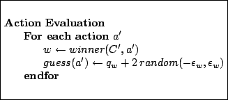
Figure 13 summarizes the action-evaluation procedure using partial rules. The value for each action is guessed using the most relevant rule for this action (i.e., the winner rule). This winner rule is computed as

winner $(C',a)=$arg $\underset{\forall w \in C'(a)}{\max}\{\rho_w\}$,

where $\rho_w$ is the relevance of rule $w$

$$\rho_w = \frac{1}{1+\epsilon_w}.$$

The value estimation using the winner rule is selected at random (uniformly) from the interval

$$I_w = [ q_w - 2 \epsilon_w,q_w + 2 \epsilon_w ],$$

with

$$\epsilon_w = e_w \: c_w + \overline{e} \: (1-c_w).$$

Here, $\overline{e}$ is the average error on the value prediction (i.e., the value error prediction of the empty rule, $w_\emptyset$).

Statistics Update

In the statistics-update procedure (Figure 14), $q_w$ and $e_w$ are adjusted for all rules that were active in the previous time step and proposed a partial command in accordance with $a$ (the last executed action).

Figure 14: Statistics update procedure.

Both $q_w$ and $e_w$ are updated using a learning rate ($m_w$) computed using the MAM function, which initially is 1, and consequently, the initial values of $q_w$ and $e_w$ have no influence on the future values of these variables. These initial values become relevant when using a constant learning rate, as many existing reinforcement-learning algorithms do.

If the observed effects of the last executed action agree with the current estimated interval for the value ($I_w$), then the confidence index is increased by one unit. Otherwise, the confidence index is decreased allowing a faster adaptation of the statistics to the last obtained, surprising values of reward.

Partial-Rule Management

This procedure (Figure 15) includes the generation of new partial rules and the removal of previously generated ones that proved to be useless.

In our implementation, we apply a heuristic that produces the generation of new partial rules when the value prediction error exceeds $\overline{e}$. In this way, we concentrate our efforts to improve the categorization on those situations with larger errors in the value prediction.

Every time a wrong prediction is made, at most $\tau$ new partial rules are generated by combination of pairs of rules included in the set $C'_{ant}(a)$. Recall that this set includes the rules active in the previous time step and in accordance with the executed action $a$. Thus, these are the rules related with the situation-action whose value prediction we need to improve.

The combination of two partial rules $w_{1} \oplus w_{2}$ consists of a new partial rule with a partial view that includes all the features included in the partial views of either $w_{1}$ or $w_{2}$ and with a partial command that includes all the elementary actions of the partial commands of either $w_{1}$ or $w_{2}$. In other words, the feature set of $w_{1} \oplus w_{2}$ is the union of the feature sets in $w_{1}$ and in $w_{2}$ and the elementary actions in $w_{1} \oplus w_{2}$ are the union of those in $w_{1}$ and those in $w_{2}$. Note that, since both $w_{1}$ and $w_{2}$ are in $C'_{ant}(a)$, they have been simultaneously active and they are in accordance with the same action and, thus, they can not be incompatible (i.e., they can not include inconsistent features or elementary actions).

Figure 15: Partial Rule Management procedure. The value of $q$ is calculated in the Statistics Update procedure and $a$ is the last executed action.

In the partial-rule creation, we bias our system to favor the combination of those rules ($w_{i}$) whose value prediction ($q_{w_{i}}$) is closer to the observed one ($q$). Finally, the generation of rules lexicographically equivalent to already existing ones is not allowed.

According to the categorizability assumption, only low-order partial rules are required to achieve the task at hand. For this reason, to improve efficiency, we limit the number of partial rules to a maximum of $\mu$. However, our partial-rule generation procedure is always generating new rules (concentrating on those situations with larger error). Therefore, when we need to create new rules and there is no room for them, we must eliminate the less useful partial rules.

A partial rule can be removed if its value prediction is too similar to some other rule in the same situations.

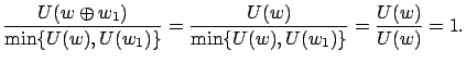
The similarity between two rules can be measured using the normalized degree of intersection between their value distributions and the number of times both rules are used simultaneously:

$$similarity(w,w')=\frac{\Vert I_w \cap I_{w'}\Vert}{\max\{\Vert I_w\Vert,\Vert I_{w'}\Vert\}} \frac{U(w \oplus w')}{\min\{U(w),U(w')\}},$$

where $U(w)$ indicates the number of times rule $w$ is actually used.

The similarity assessment for any pair of partial rules in the controller is too expensive and, in general, determining the similarity of each rule with respect to those from which it was generated (that are the rules we tried to refine when the new rule was created) is sufficient. Thus, based on the above similarity measure, we define the redundancy of a partial rule $w=(w_{1} \oplus w_{2})$ as:

$$redundancy(w)=\max\{similarity(w,w_1),similarity(w,w_2)\}.$$

Observe that with $w=(w_{1} \oplus w_{2})$, we have that $w \oplus w_{1}=w$ and $U(w) \leq U(w_1)$. Therefore

$$\frac{U(w \oplus w_1)}{\min\{U(w),U(w_1)\}}=\frac{U(w)}{\min\{U(w),U(w_1)\}}=\frac{U(w)}{U(w)}=1.$$

The same reasoning can be done with $w_2$ and, consequently,

$$redundancy(w)=\max\{\frac{\Vert I_w \cap I_{w_1}\Vert}{\max\{\Ver... ...frac{\Vert I_w \cap I_{w_2}\Vert}{\max\{\Vert I_w\Vert,\Vert I_{w_2}\Vert\}}\}.$$

When we need to create new rules but the maximum number of rules ($\mu$) has been reached, the partial rules with a redundancy above a given threshold ($\lambda$) are eliminated. Since the redundancy of a partial rule can only be estimated after observing it a number of times, the redundancy of the partial rules with low confidence indexes are set to 0, so that they are not immediately removed after creation.

Observe that, to compute the redundancy of a rule $w$, we use the partial rules from which $w$ was derived. For this reason, a rule $w'$ cannot be removed from a controller $C$ if there exists any rule $w \in C$ such that $w=w' \oplus w''$. Additionally, in this way we eliminate first the useless rules with higher order.