6 Results

Each of the 33 evolution runs took between 5 and 10 days on a 1GHz Pentium III processor, depending on the progress of evolution and sizes of the networks involved. The NEAT algorithm itself used less than 1% of this computation: Most of the time was spent in evaluating networks in the robot duel task. Evolution of fully-connected topologies took about 90% longer than structure-growing NEAT because larger networks take longer to evaluate.

In order to analyze the results, we define complexity as the number of nodes and connections in a network: The more nodes and connections there are in the network, the more complex behavior it can potentially implement. The results were analyzed to answer three questions: (1) As evolution progresses does it also continually complexify? (2) Does such complexification lead to more sophisticated strategies? (3) Does complexification allow better strategies to be discovered than does evolving fixed-topology networks? Each question is answered in turn below.

6.1 Evolution of Complexity

NEAT was run thirteen times, each time from a different seed, to verify that the results were consistent. The highest levels of dominance achieved were 17, 14, 17, 16, 16, 18, 19, 15, 17, 12, 12, 11, and 13, averaging at 15.15 (sd = 2.54).

Figure 5. Complexification of connections and nodes over generations. The hashed lines depict the average number of connections and the average number of hidden nodes in the highest dominant network in each generation. Averages are taken over 13 complexifying runs. A hash mark appears every generation in which a new dominant strategy emerged in at least one of the 13 runs. The graphs show that as dominance increases, so does complexity. The differences between the average final and first dominant strategies are statistically significant for both connections and nodes ($p < 0.001$). For comparison the dashed lines depict the sizes of the average smallest and largest networks in the entire population over five runs where the fitness is assigned randomly. These bounds show that the increase in complexity is not inevitable; both very simple and very complex species exist in the population throughout the run. When the dominant networks complexify, they do so because it is beneficial.

At each generation where the dominance level increased in at least one of the thirteen runs, we averaged the number of connections and number of nodes in the current dominant strategy across all runs (Figure 5). Thus, the graphs represent a total of 197 dominance transitions spread over 500 generations. The rise in complexity is dramatic, with the average number of connections tripling and the average number of hidden nodes rising from 0 to almost six. In a smooth trend over the first 200 generations, the number of connections in the dominant strategy grows by 50%. During this early period, dominance transitions occur frequently (fewer prior strategies need to be beaten to achieve dominance). Over the next 300 generations, dominance transitions become more sparse, although they continue to occur.

Between the 200th and 500th generations a stepped pattern emerges: The complexity first rises dramatically, then settles, then abruptly increases again (This pattern is even more marked in individual complexifying runs; the averaging done in Figure 5 smooths it out somewhat). The cause for this pattern is speciation. While one species is adding a large amount of structure, other species are optimizing the weights of less complex networks. Initially, added complexity leads to better performance, but subsequent optimization takes longer in the new higher-dimensional space. Meanwhile, species with smaller topologies have a chance to temporarily catch up through optimizing their weights. Ultimately, however, more complex structures eventually win, since higher complexity is necessary for continued innovation.

Thus, there are two underlying forces of progress: The building of new structures, and the continual optimization of prior structures in the background. The product of these two trends is a gradual stepped progression towards increasing complexity.

An important question is: Because NEAT searches by adding structure only, not by removing it, does the complexity always increase whether it helps in finding good solutions or not? To demonstrate that NEAT indeed prefers simple solutions and complexifies only when it is useful, we ran five complexifying evolution runs with fitness assigned randomly (i.e. the winner of each game was chosen at random). As expected, NEAT kept a wide range of networks in its population, from very simple to highly complex (Figure 5). That is, the dominant networks did not have to become more complex; they only did so because it was beneficial. Not only is the minimum complexity in the random-fitness population much lower than that of the dominant strategies, but the maximum complexity is significantly greater. Thus, evolution complexifies sparingly, only when the complex species holds its own in comparison with the simpler ones.

6.2 Sophistication through Complexification

To see how complexification contributes to evolution, let us observe how a sample dominant strategy develops over time. While many complex networks evolved in the experiments, we follow the species that produced the winning network $d_{17}$ in the third run because its progress is rather typical and easy to understand. Let us use $S_k$ for the best network in species $S$ at generation $k$, and $h_l$ for the $l$th hidden node to arise from a structural mutation over the course of evolution. We will track both strategic and structural innovations in order to see how they correlate. Let us begin with $S_{100}$ (Figure 6a), when $S$ had a mature zero-hidden-node strategy:

• $S_{100}$'s main strategy was to follow the opponent, putting it in a position where it might by chance collide with its opponent when its energy is up. However, $S_{100}$ followed the opponent even when the opponent had more energy, leaving $S_{100}$ vulnerable to attack. $S_{100}$ did not clearly switch roles between foraging and chasing the enemy, causing it to miss opportunities to gather food.

• $S_{200}$. During the next 100 generations, $S$ evolved a resting strategy, which it used when it had significantly lower energy than its opponent. In such a situation, the robot stopped moving, while the other robot wasted energy running around. By the time the opponent got close, its energy was often low enough to be attacked. The resting strategy is an example of improvement that can take place without complexification: It involved increasing the inhibition from the energy difference sensor, thereby slightly modifying intensity of an existing behavior.

• In $S_{267}$ (Figure 6b), a new hidden node, $h_{22}$, appeared. This node arrived through an interspecies mating, and had been optimized for several generations already. Node $h_{22}$ gave the robot the ability to change its behavior at once into an all-out attack. Because of this new skill, $S_{267}$ no longer needed to follow the enemy closely at all times, allowing it to collect more food. By implementing this new strategy through a new node, it was possible not to interfere with the already existing resting strategy, so that $S$ now switched roles between resting when at a disadvantage to attacking when high on energy. Thus, the new structure resulted in strategic elaboration.

• In $S_{315}$ (Figure 6c), another new hidden node, $h_{172}$, split a link between an input sensor and $h_{22}$. Replacing a direct connection with a sigmoid function greatly improved $S_{315}$'s ability to attack at appropriate times, leading to very accurate role switching between attacking and foraging. $S_{315}$ would try to follow the opponent from afar focusing on resting and foraging, and only zoom in for attack when victory was certain. This final structural addition shows how new structure can improve the accuracy and timing of existing behaviors.

The analysis above shows that in some cases, weight optimization alone can produce improved strategies. However, when those strategies need to be extended, adding new structure allows the new behaviors to coexist with old strategies. Also, in some cases it is necessary to add complexity to make the timing or execution of the behavior more accurate. These results show how complexification can be utilized to produce increasing sophistication.

In order to illustrate the level of sophistication achieved in this process, we conclude this section by describing the competition between two sophisticated strategies, $S_{210}$ and $S_{313}$, from another run of evolution. At the beginning of the competition, $S_{210}$ and $S_{313}$ collected most of the available food until their energy levels were about equal. Two pieces of food remained on the board in locations distant from both $S_{210}$ and $S_{313}$ (Figure 7). Because of the danger of colliding with similar energy levels, the obvious strategy is to rush for the last two pieces of food. In fact, $S_{210}$ did exactly that, consuming the second-to-last piece, and then heading towards the last one. In contrast, $S_{313}$ forfeited the race for the second-to-last piece, opting to sit still, even though its energy temporarily dropped below $S_{210}$'s. However, $S_{313}$ was closer to the last piece and got there first. It received a boost of energy while $S_{210}$ wasted its energy running the long distance from the second-to-last piece. Thus, $S_{313}$'s strategy ensured that it had more energy when they finally met. Robot $S_{313}$'s behavior was surprisingly deceptive, showing that high strategic sophistication had evolved. Similar waiting behavior was observed against several other opponents, and also evolved in several other runs, suggesting that it was a robust result.

This analysis of individual evolved behaviors shows that complexification indeed elaborates on existing strategies, and allows highly sophisticated behaviors to develop that balance multiple goals and utilize weaknesses in the opponent. The last question is whether complexification indeed is necessary to achieve these behaviors.

6.3 Complexification vs. Fixed-topology Evolution and Simplification

Complexifying coevolution was compared to two alternatives: standard coevolution in a fixed search space, and to simplifying coevolution from a complex starting point. Note that it is not possible to compare methods using the standard crossvalidation techniques because no external performance measure exists in this domain. However, the evolved neural networks can be compared directly by playing a duel. Thus, for example, a run of fixed-topology coevolution can be compared to a run of complexifying coevolution by playing the highest dominant strategy from the fixed-topology run against the entire dominance ranking of the complexifying run. The highest level strategy in the ranking that the fixed-topology strategy can defeat, normalized by the number of dominance levels, is a measure of its quality against the complexifying coevolution. For example, if a strategy can defeat up to and including the 13th dominant strategy out of 15, then its performance against that run is $\frac{13}{15}=86.7\%$. By playing every fixed-topology champion, every simplifying coevolution champion, and every complexifying coevolution champion against the dominance ranking from every complexifying run and averaging, we can measure the relative performance of each of these methods.

In this section, we will first establish the baseline performance by playing complexifying coevolution runs against themselves and demonstrating that a comparison with dominance levels is a meaningful measure of performance. We will then compare complexification with fixed-topology coevolution of networks of different architectures, including fully-connected small networks, fully-connected large networks, and networks with an optimal structure as determined by complexifying coevolution. Third, we will compare the performance of complexification with that of simplifying coevolution.

6.3.1 Complexifying Coevolution

The highest dominant strategy from each of the 13 complexifying runs played the entire dominance ranking from every other run. Their average performance scores were $87.9\%$, $83.8\%$, $91.9\%$, $79.4\%$, $91.9\%$, $99.6\%$, $99.4\%$, $99.5\%$, $81.8\%$, $96.2\%$, $90.6\%$, $96.9\%$, and $89.3\%$, with an overall average of $91.4\%$ (sd=12.8%). Above all, this result shows that complexifying runs produce consistently good strategies: On average, the highest dominant strategies qualify for the top $10\%$ of the other complexifying runs. The best runs were the sixth, seventh, and eighth, which were able to defeat almost the entire dominance ranking of every other run. The highest dominant network from the best run ($99.6\%$) is shown in Figure 8.

In order to understand what it means for a network to be one or more dominance levels above another, figure 9 shows how many more games the more dominant network can be expected to win on average over all its 288-game comparisons than the less dominant network. Even at the lowest difference (i.e. that of one dominance level), the more dominant network can be expected to win about 50 more games on average, showing that each difference in dominance level is important. The difference grows approximately linearly: A network 5 dominance levels higher will win 100 more games, while a network 10 levels higher will win 150 and 15 levels higher will win 200. These results suggest that dominance level comparisons indeed constitute a meaningful way to measure relative performance.

6.3.2 Fixed-Topology Coevolution of Large Networks

In fixed-topology coevolution, the network architecture must be chosen by the experimenter. One sensible approach is to approximate the complexity of the best complexifying network. (Figure 8). This network included 11 hidden units and 202 connections, with both recurrent connections and direct connections from input to output. As an idealization of this structure, we used 10-hidden-unit fully recurrent networks with direct connections from inputs to outputs, with a total of 263 connections. A network of this type should be able to approximate the functionality of the most effective complexifying strategy. Fixed-topology coevolution runs exactly as complexifying coevolution in NEAT, except that no structural mutations can occur. In particular, the population is still speciated based on weight differences (i.e. $\overline{W}$ from equation 1), using the usual speciation procedure.

Three runs of fixed-topology coevolution were performed with these networks, and their highest dominant strategies were compared to the entire dominance ranking of every complexifying run. Their average performances were $29.1\%$, $34.4\%$, and $57.8\%$, for an overall average of $40.4\%$. Compared to the $91.4\%$ performance of complexifying coevolution, it is clear that fixed-topology coevolution produced consistently inferior solutions. As a matter of fact, no fixed-topology run could defeat any of the highest dominant strategies from the 13 complexifying coevolution runs.

This difference in performance can be illustrated by computing the average generation of complexifying coevolution with the same performance as fixed-topology coevolution. This generation turns out to be 24 (sd = 8.8). In other words, 500 generations of fixed-topology coevolution reach on average the same level of dominance as only 24 generations of complexifying coevolution! In effect, the progress of the entire fixed-topology coevolution run is compressed into the first few generations of complexifying coevolution (Figure 10).

6.3.3 Fixed-Topology Coevolution of Small Networks

One of the arguments for using complexifying coevolution is that starting the search directly in the space of the final solution may be intractable. This argument may explain why the attempt to evolve fixed-topology solutions at a high level of complexity failed. Thus, in the next experiment we aimed at reducing the search space by evolving fully-connected, fully-recurrent networks with a small number of hidden nodes as well as direct connections from inputs to outputs. After considerable experimentation, we found out that five hidden nodes (144 connections) was appropriate, allowing fixed-topology evolution to find the best solutions it could. Five hidden nodes is also about the same number of hidden nodes as the highest dominant strategies had on average in the complexifying runs.

A total of seven runs were performed with the 5-hidden-node networks, with average performances of $70.7\%$, $85.5\%$, $66.1\%$, $87.3\%$, $80.8\%$, $88.8\%$, and $83.1\%$. The overall average was $80.3\%$ (sd=18.4%), which is better but still significantly below the $91.4\%$ performance of complexifying coevolution ($p < 0.001$).

In particular, the two most effective complexifying runs were still never defeated by any of the fixed-topology runs. Also, because each dominance level is more difficult to achieve than the last, on average the fixed-topology evolution only reached the performance of the 159th complexifying generation (sd=72.0). Thus, even in the best case, fixed-topology coevolution on average only finds the level of sophistication that complexifying coevolution finds halfway through a run (Figure 11).

6.3.4 Fixed-Topology Coevolution of Best Complexifying Network

One problem with evolving fully-connected architectures is that they may not have an appropriate topology for this domain. Of course, it is very difficult to guess an appropriate topology a priori. However, it is still interesting to ask whether fixed-topology coevolution could succeed in the task assuming that the right topology was known? To answer this question, we evolved networks as in the other fixed-topology experiments, except this time using the topology of the best complexifying network (Figure 8). This topology may constrain the search space in such a way that finding a sophisticated solution is more likely than with a fully-connected architecture. If so, it is possible that seeding the population with a successful topology gives it an advantage even over complexifying coevolution, which must build the topology from a minimal starting point.

Five runs were performed, obtaining average performance score $86.2\%$, $83.3\%$, $88.1\%$, $74.2\%$, and $80.3\%$, and an overall average of $82.4\%$ (sd=$15.1\%$). The $91.4\%$ performance of complexifying coevolution is significantly better than even this version of fixed-topology coevolution ($p < 0.001$). However, interestingly, the $40.4\%$ average performance of 10-hidden-unit fixed topology coevolution is significantly below best-topology evolution, even though both methods search in spaces of similar sizes. In fact, best-topology evolution performs at about the same level as 5-hidden-unit fixed-topology evolution ($80.3\%$), even though 5-hidden-unit evolution optimizes half the number of hidden nodes. Thus, the results confirm the hypothesis that using a successful evolved topology does help constrain the search. However, in comparison to complexifying coevolution, the advantage gained from starting this way is still not enough to make up for the penalty of starting search directly in a high-dimensional space. As Figure 12 shows, best-topology evolution on average only finds a strategy that performs as well as those found by the 193rd generation of complexifying coevolution.

The results of the fixed-topology coevolution experiments can be summarized as follows: If this method is used to search directly in the high-dimensional space of the most effective solutions, it reaches only 40% of the performance of complexifying coevolution. It does better if it is allowed to optimize less complex networks; however, the most sophisticated solutions may not exist in that space. Even given a topology appropriate for the task, it does not reach the same level as complexifying coevolution. Thus, fixed-topology coevolution does not appear to be competitive with complexifying coevolution with any choice of topology.

The conclusion is that complexification is superior not only because it allows discovering the appropriate high-dimensional topology automatically, but also because it makes the optimization of that topology more efficient. This point will be discussed further in Section 7.

6.3.5 Simplifying Coevolution

A possible remedy to having to search in high-dimensional spaces is to allow evolution to search for smaller structures by removing structure incrementally. This simplifying coevolution is the opposite of complexifying coevolution. The idea is that a mediocre complex solution can be refined by removing unnecessary dimensions from the search space, thereby accelerating the search.

Although simplifying coevolution is an alternative method to complexifying coevolution for finding topologies, it still requires a complex starting topology to be specified. This topology was chosen with two goals in mind: (1) Simplifying coevolution should start with sufficient complexity to at least potentially find solutions of equal or more complexity than the best solutions from complexifying coevolution, and (2) with a rate of structural removal equivalent to the rate of structural addition in complexifying NEAT, it should be possible to discover solutions significantly simpler than the best complexifying solutions. Thus, we chose to start search with a 12-hidden-unit, 339 connection fully-connected fully-recurrent network. Since 162 connections were added to the best complexifying network during evolution, a corresponding simplifying coevolution could discover solutions with 177 connections, or 25 less than the best complexifying network.

Thus, simplify coevolution was run just as complexifying coevolution, except that the initial topology contained 339 connections instead of 39, and structural mutations removed connections instead of adding nodes and connections. If all connections of a node were removed, the node itself was removed. Historical markings and speciation worked as in complexifying NEAT, except that all markings were assigned in the beginning of evolution. (because structure was only removed and never added). A diversity of species of varying complexity developed as before.

The five runs of simplifying coevolution performed at $64.8\%$, $60.9\%$, $56.6\%$, $36.4\%$, and $67.9\%$, with an overall average of $57.3\%$ (sd=19.8%). Again, such performance is significantly below the $91.4\%$ performance of complexifying coevolution ($p < 0.001$). Interestingly, even though it started with 76 more connections than fixed-topology coevolution with ten hidden units, simplifying coevolution still performed significantly better ($p < 0.001$), suggesting that evolving structure through reducing complexity is better than evolving large fixed structures.

Like Figures 10-12, Figure 13 compares typical runs of complexifying and simplifying coevolution. On average, 500 generations of simplification finds solutions equivalent to 56 generations of complexification. Simplifying coevolution also tends to find more dominance levels than any other method tested. It generated an average of $23.2$ dominance levels per run, once even finding $30$ in one run, whereas e.g. complexifying coevolution on average finds $15.2$ levels. In other words, the difference between dominance levels is much smaller in simplifying coevolution than complexifying coevolution. Unlike in other methods, dominant strategies tend to appear in spurts of a few at a time, and usually after complexity has been decreasing for several generations, as also shown in Figure 13. Over a number of generations, evolution removes several connections until a smaller, more easily optimized space is discovered. Then, a quick succession of minute improvements creates several new levels of dominance, after which the space is further refined, and so on. While such a process makes sense, the inferior results of simplifying coevolution suggest that simplifying search is an ineffective way of discovering useful structures compared to complexification.

6.3.6 Comparison Summary

Table 1: Summary of the performance comparison. The second column shows how many levels of dominance were achieved in each type of coevolution on average. The third specifies the average generation of the highest dominant strategy, indicating how long innovation generally continues. The fourth column gives the average level in the complexifying coevolution dominance hierarchy that the champion could defeat, and the fifth column shows its average generation. The differences in performance ($p < 0.001$) and equivalent generation ($p < 0.001$) between complexifying coevolution and every other method are significant. The main result is that the level of sophistication reached by complexifying coevolution is significantly higher than that reached by fixed-topology or simplifying coevolution.

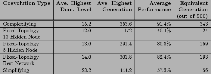
Table 1 shows how the coevolution methods differ on number of dominance levels, generation of the highest dominance level, overall performance, and equivalent generation. The conclusion is that complexifying coevolution innovates longer and finds a higher level of sophistication than the other methods.