 |
To get some intuition about the performance of the algorithm we created
a ring (one large loop) of 200 binary nodes. Nodes are connected as in
the Boltzmann machine with a weight ![]() and each node has a threshold
and each node has a threshold
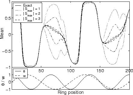
![]() . Weights and thresholds are varying along the ring as is shown
at the bottom of Figure
. Weights and thresholds are varying along the ring as is shown
at the bottom of Figure ![[*]](crossref.png) . For this simple problem we can compute
the exact single node marginals. These are plotted as a solid line in
Figure . We ran the bound propagation algorithm
three times, where we varied the maximum
number of nodes included in
. For this simple problem we can compute
the exact single node marginals. These are plotted as a solid line in
Figure . We ran the bound propagation algorithm
three times, where we varied the maximum
number of nodes included in
![]() :
:
![]() ,
,
![]() and
and
![]() . In all cases
we chose two separator nodes: the two neighbors of
. In all cases
we chose two separator nodes: the two neighbors of
![]() . Thus these
three cases correspond to
. Thus these
three cases correspond to
![]() ,
,
![]() and
and
![]() . As is clear from Figure the simplest
choice already find excellent bounds for the majority of the nodes.
For large negative weights, however, this choice is not sufficient.
Allowing larger separators clearly improves the result. In all cases
the computation time was a few seconds2.
. As is clear from Figure the simplest
choice already find excellent bounds for the majority of the nodes.
For large negative weights, however, this choice is not sufficient.
Allowing larger separators clearly improves the result. In all cases
the computation time was a few seconds2.